| wais | senility |
|---|---|
| 9 | 1 |
| 13 | 1 |
| 6 | 1 |
| 8 | 1 |
| 10 | 1 |
| 4 | 1 |
Write Up Example & Block 4 Recap
Learning Objectives
At the end of this lab, you will:
- Understand how to write-up and provide interpretation of a binary logistic regression model
What You Need
- Be up to date with lectures
- Have completed Labs 7-9
Required R Packages
Remember to load all packages within a code chunk at the start of your RMarkdown file using library(). If you do not have a package and need to install, do so within the console using install.packages(" "). For further guidance on installing/updating packages, see Section C here.
For this lab, you will need to load the following package(s):
- tidyverse
- psych
- kableExtra
- sjPlot
Lab Data
You can download the data required for this lab here or read it in via this link https://uoepsy.github.io/data/SenilityWAIS.csv.
Section A: Write-Up
In this section of the lab you will be be presented with a research question, and tasked with writing up and presenting your analyses.
The aim in writing should be that a reader is able to more or less replicate your analyses without referring to your R code. This requires detailing all of the steps you took in conducting the analysis. The point of using RMarkdown is that you can pull your results directly from the code. If your analysis changes, so does your report!
Make sure that your final report doesn’t show any R functions or code. Remember you are interpreting and reporting your results in text, tables, or plots, targeting a generic reader who may use different software or may not know R at all. If you need a reminder on how to hide code, format tables, etc., make sure to review the rmd bootcamp.
The example write-up sections included below are not perfect - they instead should give you a good example of what information you should include within each section, and how to structure this. For example, some information is missing (e.g., interpretation of descriptive statistics, what type of interaction is present), some information could be presented more clearly (e.g., variable names in tables, table/figure titles/captions, and rationales for choices), and writing could be more concise in places (e.g., discussion section is quite long).
Further, you must not copy any of the write-up included below for future reports - if you do, you will be committing plagiarism, and this type of academic misconduct is taken very seriously by the University. You can find out more here.
Study Overview
Research Question
Does the probability of having senility symptoms change as a function of the WAIS score?
Description
A sample of elderly people was given a psychiatric examination to determine if symptoms of senility were present. Other measurements taken at the same time included the score on a subset of the Wechsler Adult Intelligence Scale (WAIS).
The data in SenilityWAIS.csv contain two attributes collected from a sample of \(n=54\) participants:
-
wais: Score on WAIS -
senility: Whether symptoms of senility were (senility = 1) or were not (senility = 0) present
Preview
The first six rows of the data are:
Setup
- Create a new RMarkdown file
- Load the required package(s)
- Read the SenilityWAIS dataset into R, assigning it to an object named
sen
Analysis Code
Try to answer the research question above without referring to the provided analysis code below, and then check how your script matches up - is there anything you missed or done differently? If so, discuss the differences with a tutor - there are lots of ways to code to the same solution!
######Step 1 is always to read in the data, then to explore, check, describe, and visualise it.

#check coding of variables - are they coded as they should be?
str(sen)
spc_tbl_ [54 × 2] (S3: spec_tbl_df/tbl_df/tbl/data.frame)
$ wais : num [1:54] 9 13 6 8 10 4 14 8 11 7 ...
$ senility: num [1:54] 1 1 1 1 1 1 1 1 1 1 ...
- attr(*, "spec")=
.. cols(
.. wais = col_double(),
.. senility = col_double()
.. )
- attr(*, "problems")=<externalptr> head(sen)# A tibble: 6 × 2
wais senility
<dbl> <dbl>
1 9 1
2 13 1
3 6 1
4 8 1
5 10 1
6 4 1#both variables currently coded as should be - no changes needed.
#create descriptives table
descript <- sen %>%
group_by(senility) %>%
summarise(
Mean_WAIS = mean(wais),
SD_WAIS = sd(wais),
Min_WAIS = min(wais),
Max_WAIS = max(wais)) %>%
kable(caption = "Descriptive Statistics", digits = 2) %>%
kable_styling()
descript| senility | Mean_WAIS | SD_WAIS | Min_WAIS | Max_WAIS |
|---|---|---|---|---|
| 0 | 12.50 | 3.46 | 4 | 20 |
| 1 | 8.93 | 3.17 | 4 | 14 |
#bar plot - senility presence
sen_plt1 <- ggplot(data = sen, aes(x = as_factor(senility), fill = as_factor(senility))) +
  geom_bar() +
    labs(x = "Senility Symptoms Present (0 = No, 1 = Yes)", fill = "Senility Symptoms Present \n(0 = No, 1 = Yes)", y = "Frequency")
sen_plt1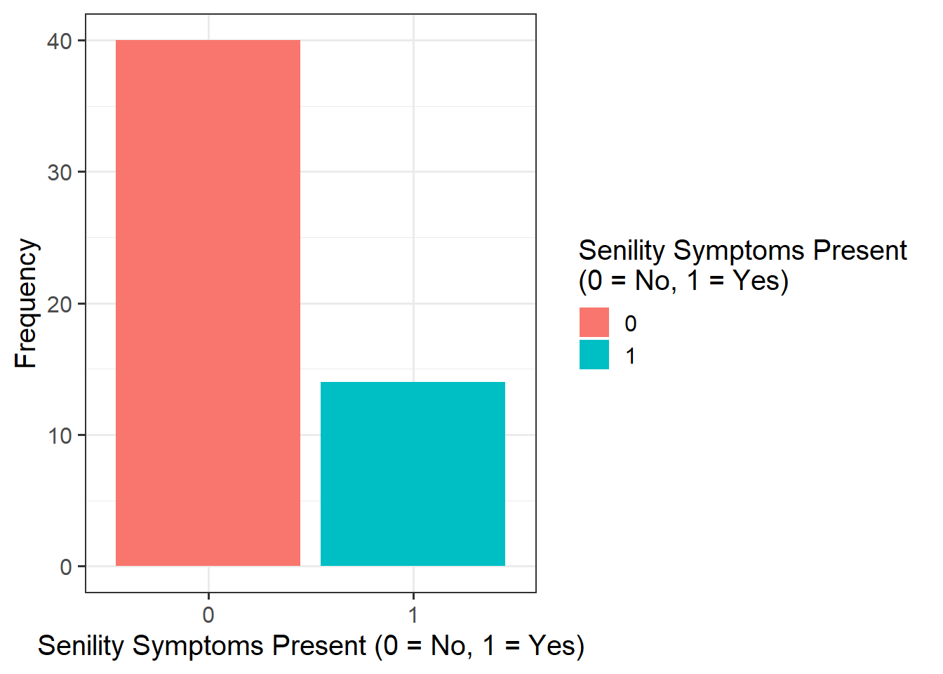
#density plot - senility & WAIS
sen_plt2 <- ggplot(data = sen, aes(x = wais, fill = as_factor(senility))) +
  geom_density() +
    labs(x = "WAIS Score", fill = "Senility Symptoms Present \n(0 = No, 1 = Yes)")
sen_plt2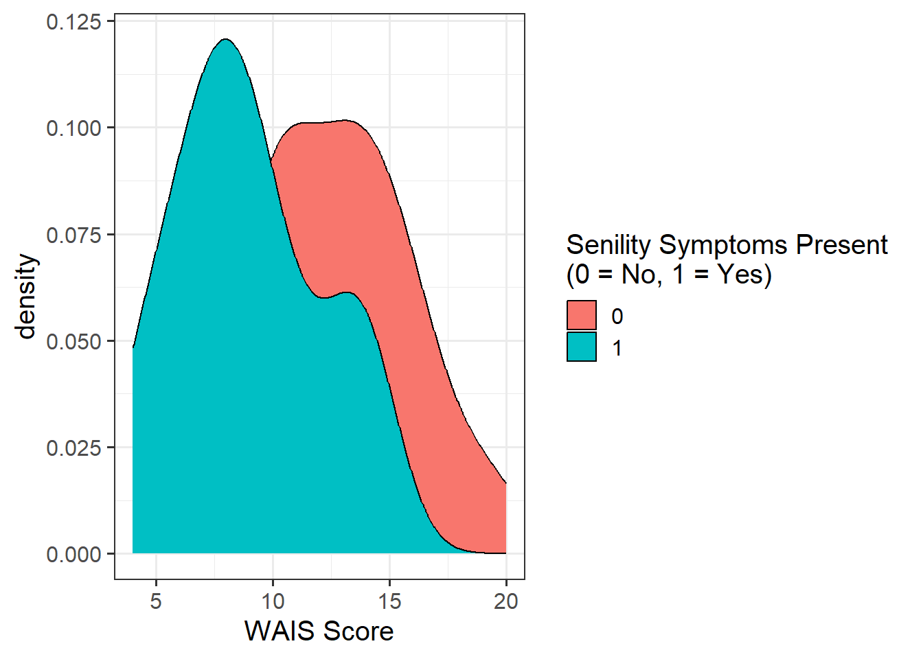
######Step 2 is to run your model(s) of interest to answer your research question, and make sure that the data meet the assumptions of your chosen test

#build model & examine output
sen_mdl1 <- glm(senility ~ wais, family = "binomial", data = sen)
summary(sen_mdl1)
Call:
glm(formula = senility ~ wais, family = "binomial", data = sen)

Deviance Residuals:
    Min       1Q   Median       3Q      Max
-1.6702  -0.7402  -0.4749   0.5200   2.1157

Coefficients:
            Estimate Std. Error z value Pr(>|z|)
(Intercept)   2.4040     1.1918   2.017  0.04369 *
wais         -0.3235     0.1140  -2.838  0.00453 **
---
Signif. codes:  0 '***' 0.001 '**' 0.01 '*' 0.05 '.' 0.1 ' ' 1

(Dispersion parameter for binomial family taken to be 1)

    Null deviance: 61.806  on 53  degrees of freedom
Residual deviance: 51.017  on 52  degrees of freedom
AIC: 55.017

Number of Fisher Scoring iterations: 5exp(coefficients(sen_mdl1))(Intercept) wais
11.06784 0.72359 #check model fit
plot(rstandard(sen_mdl1, type = "deviance"), ylab = "Standardised Deviance Residuals")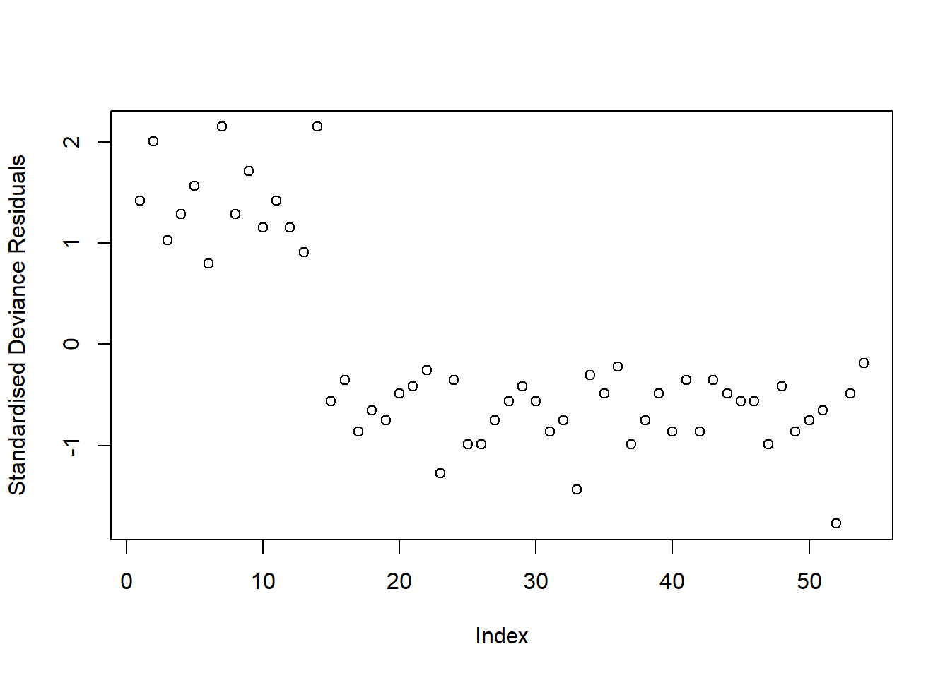
plot(cooks.distance(sen_mdl1), ylab = "Cook's Distance")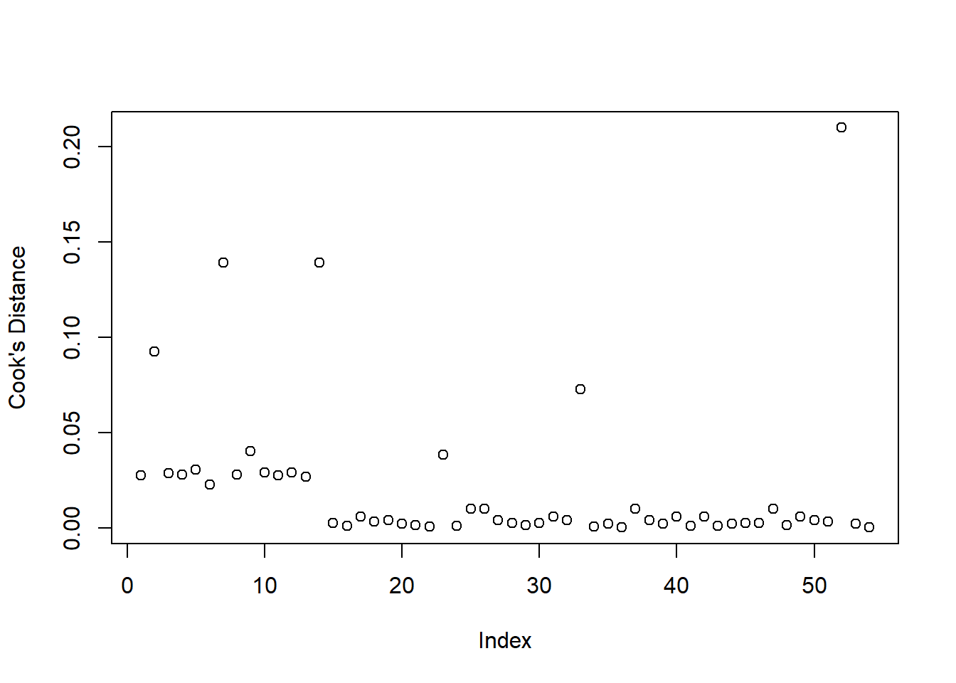
#compare to null - conduct model comparison
#fit null
sen_mdl0 <- glm(senility ~ 1, family = "binomial", data = sen)
#compare models - models are nested
anova(sen_mdl0, sen_mdl1, test = "Chisq")
Analysis of Deviance Table
Model 1: senility ~ 1
Model 2: senility ~ wais
Resid. Df Resid. Dev Df Deviance Pr(>Chi)
1 53 61.806
2 52 51.017 1 10.789 0.001021 **
---
Signif. codes: 0 '***' 0.001 '**' 0.01 '*' 0.05 '.' 0.1 ' ' 1AIC(sen_mdl0, sen_mdl1) df AIC
sen_mdl0 1 63.80632
sen_mdl1 2 55.01738BIC(sen_mdl0, sen_mdl1) df BIC
sen_mdl0 1 65.79530
sen_mdl1 2 58.99535#plot model
plt_mdl1 <- plot_model(sen_mdl1, type = "eff")
plt_mdl1$wais
#results in formatted table
tab_model(sen_mdl1,
          dv.labels = "Senility Symptoms",
          pred.labels = c("wais" = "WAIS"),
title = "Regression Table for Senility Model")| Senility Symptoms | |||
|---|---|---|---|
| Predictors | Odds Ratios | CI | p |
| (Intercept) | 11.07 | 1.23 – 145.24 | 0.044 |
| WAIS | 0.72 | 0.56 – 0.89 | 0.005 |
| Observations | 54 | ||
| R2 Tjur | 0.198 | ||
The 3-Act Structure: Analysis Strategy, Results, & Discussion
Recall that we need to present our report in three clear sections - think of your sections like the 3 key parts of a play or story - we need to (1) provide some background and scene setting for the reader, (2) present our results in the context of the research question, and (3) present a resolution to our story - relate our findings back to the question we were asked and provide our answer.
If you need a reminder of what to include within each section, refer to Semester 1 Lab 11, and read through the ‘what to include’ sections for Analysis Strategy, Results, and Discussion.
Act I: Analysis Strategy
Attempt to draft a discussion section based on the above research question and analysis provided.
The SenilityWAIS dataset contained information on 54 participants who took part in a study concerning the presence of senility symptoms (scored dichotomously as present (1) or not present (0). The sample of older adults also completed the Wechsler Adult Intelligence Scale (WAIS), and scores were available for a subset of these items. All participant data was complete (no missing values).
To investigate whether the probability of having senility symptoms change as a function of WAIS score, a binary logistic regression model was used. Effects were considered statistically significant at \(\alpha = .05\). The following model specification was used:
\[ \begin{aligned} M_1 &: \qquad \log \left( \frac{p}{1 - p}\right) = \beta_0 + \beta_1 \cdot \text{WAIS} \end{aligned} \]
To address the research question of whether the probability of having senility symptoms change as a function of WAIS score, this formally corresponded to testing whether the WAIS coefficient was equal to zero:
\[ H_0: \beta_1 = 0 \]
\[ H_1: \beta_1 \neq 0 \]
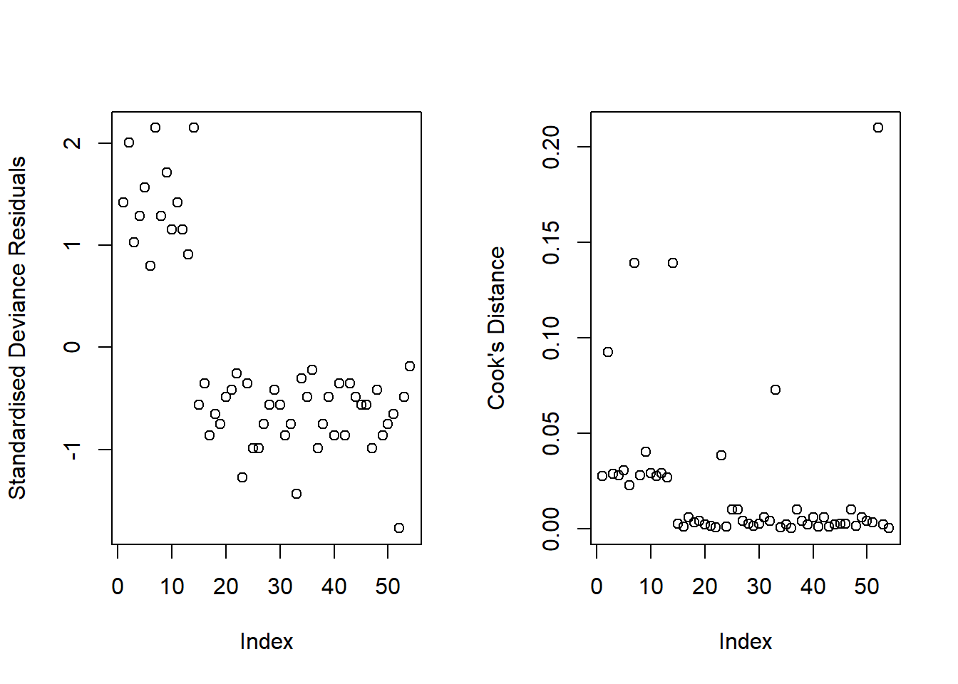
To assess model fit, we visually assessed the standardized deviance residuals and Cook’s Distance. We expected the former to identify outliers (or extreme values), and we expected residuals to fall within the range of -2 to 2. We used the latter to check for influential observations, and visually assessed if any of our 54 observations had a Cook’s distance > than 0.5 (moderately influential) or > 1 (highly influential).
Act II: Results
Attempt to draft a results section based on your detailed analysis strategy and the analysis provided.
Descriptive statistics are displayed in Table 1.
| senility | Mean_WAIS | SD_WAIS | Min_WAIS | Max_WAIS |
|---|---|---|---|---|
| 0 | 12.50 | 3.46 | 4 | 20 |
| 1 | 8.93 | 3.17 | 4 | 14 |
It appeared that there those without senility symptoms present had higher WAIS scores than those with symptoms (see Figure 1).

A binary logistic regression model was fitted to determine whether the probability of having senility symptoms change as a function of WAIS score.
Our model did not raise any concerns regarding fit. Though there appeared to be a few residuals with a value slightly larger than 2 in absolute value (see left-hand plot in Figure 2), they were not influential points (see right-hand plot in Figure 2), since none of our observations had a Cook’s distance value > 0.5.
WAIS scores were a significant predictor of whether or not individuals experienced senility symptoms (see Table 2), where for every additional point scored on the WAIS, the odds of having senility symptoms decreased by a factor of 0.72 (\(95\%\, CI\, [0.56, 0.89]\)).
| Senility Symptoms | |||
|---|---|---|---|
| Predictors | Odds Ratios | CI | p |
| (Intercept) | 11.07 | 1.23 – 145.24 | 0.044 |
| WAIS | 0.72 | 0.56 – 0.89 | 0.005 |
| Observations | 54 | ||
| R2 Tjur | 0.198 | ||
We visualised the predicted probability based on our model estimates (see Figure 3), which suggested that higher WAIS scores were associated with a lower probability of endorsing senility symptoms.
$wais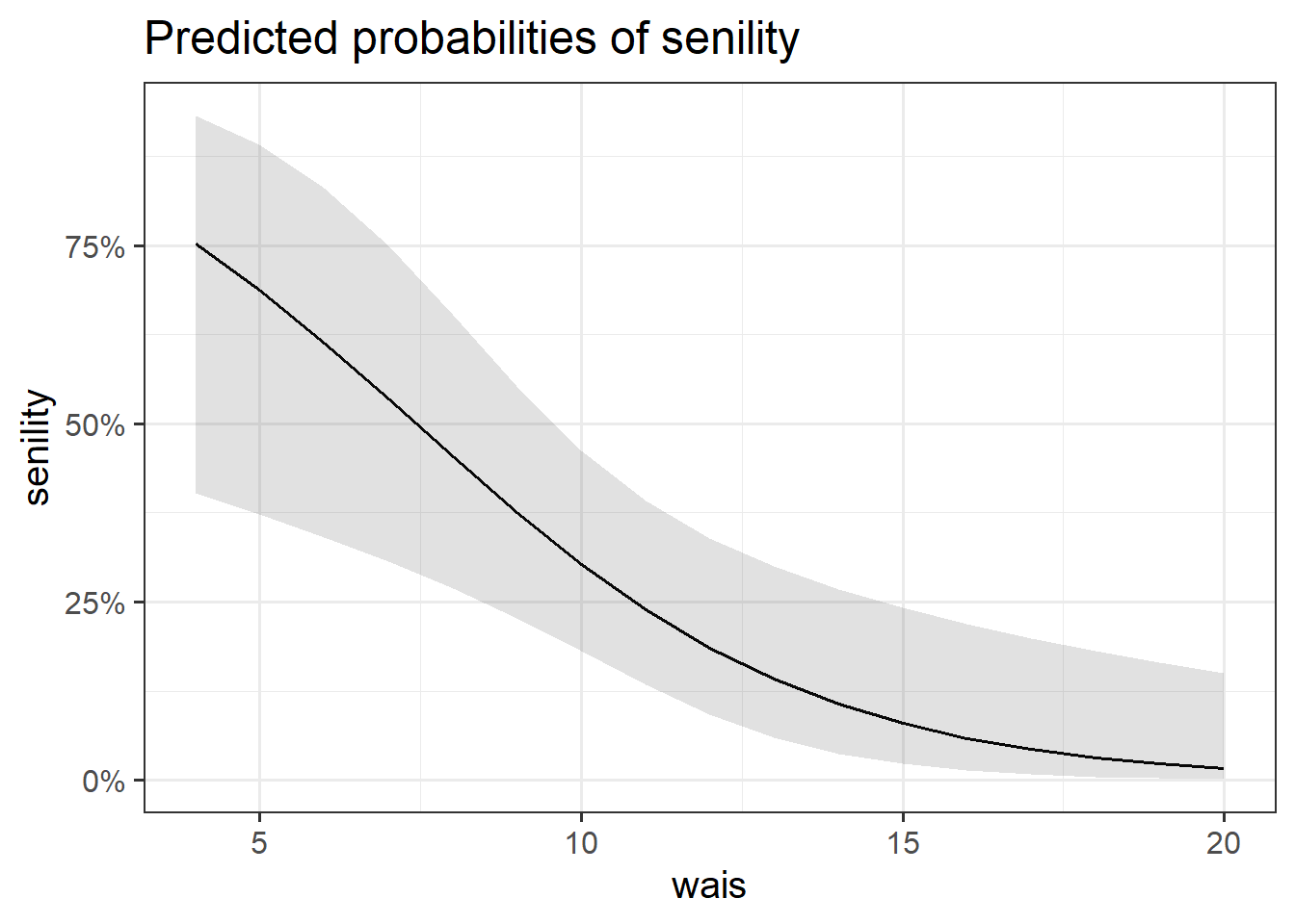
We performed a deviance goodness-of-fit test to compare our fitted model to the null. At the 5% significance level, the addition of information about the participants’ WAIS resulted in a significant decrease in model deviance \(\chi^2(1) = 10.78, p = .001\). Hence, we have strong evidence that the subjects’ WAIS was a helpful predictor of whether or not participants will experience symptoms of senility.
Act III: Discussion
Attempt to draft a discussion section based on your results and the analysis provided.
Our results led us to reject the null hypothesis, as the direction of the association was clear from the results of our binary logistic regression model - lower WAIS scores increased the odds of endorsing senility symptoms. In conclusion, the presence of senility symptoms varied as a function of WAIS score.
Section B: Weeks 6-10 Recap
In the second part of the lab, there is no new content - the purpose of the recap section is for you to revisit and revise the concepts you have learned over the last 4/5 weeks.
Before you expand each of the boxes below, think about how comfortable you feel with each concept.
The probability \(p\) ranges from 0 to 1.
The odds \(\frac{p}{1-p}\) ranges from 0 to \(\infty\).
The log-odds \(\log \left( \frac{p}{1-p} \right)\) ranges from \(-\infty\) to \(\infty\).
In the labs, we used “log” to denote log-odds. In the lectures, you will have seen this denoted as “ln”.
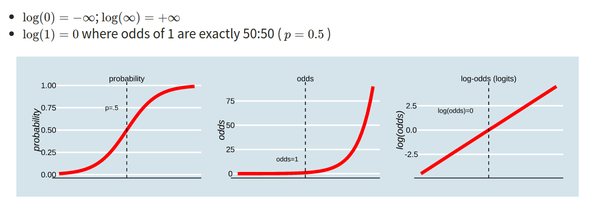
In order to understand the connections among these concepts, lets work with an example where the probability of an event occurring is 0.2:
- Odds of event occurring:
\[ \text{odds} = (\frac{0.2}{0.8}) = 0.25 \]
- Log-odds of the event occurring:
\[ log(\frac{0.2}{0.8}) = -1.3863 \\ \ \\ \]
\[ log(0.25) = -1.3863 \]
- Probability can be reconstructed as:
\[ (\frac{exp(log(odds))}{1+exp(log(odds))}) = (\frac{exp(-1.3863)}{1+exp(-1.3683)}) = (\frac{0.25}{1.25}) = 0.2 \]
In R:
-
obtain the odds
odds <- 0.2 / (1 - 0.2) -
obtain the log-odds for a given probability
log_odds <- log(0.25)OR
log_odds <- qlogis(0.2) -
obtain the probability from the odds
prob_O <- odds / (1 + odds) -
obtain the probability from the log-odds
prob_LO <- exp(log_odds) / (1 + exp(log_odds))OR
prob_LO <- plogis(log_odds)
See S2 Week 6 lecture, S2 Week 6 lab, and S2 Week 7 lab for further details, examples, and to revise these concepts further.
When a response (y) is binary coded (e.g., 0/1; failure/success; no/yes; fail/pass; unemployed/employed) we must use logistic regression. The predictors can either be continuous or categorical.
\[ {\log(\frac{p_i}{1-p_i})} = \beta_0 + \beta_1 \ x_{i1} \]
In R:
glm(y ~ x1 + x2, data = data, family = binomial)See S2 Week 6 lecture, S2 Week 6 lab, and S2 Week 7 lab for further details, examples, and to revise these concepts further.
To interpret the fitted coefficients, we first exponentiate the model: \[ \begin{aligned} \log \left( \frac{p_x}{1-p_x} \right) &= \beta_0 + \beta_1 x \\ e^{ \log \left( \frac{p_x}{1-p_x} \right) } &= e^{\beta_0 + \beta_1 x } \\ \frac{p_x}{1-p_x} &= e^{\beta_0} \ e^{\beta_1 x} \end{aligned} \]
and recall that the probability of success divided by the probability of failure is the odds of success. \[ \frac{p_x}{1-p_x} = \text{odds} \]
Let’s apply this to our lab example from Section A above:
Intercept
\[ \text{If }x = 0, \qquad \frac{p_0}{1-p_0} = e^{\beta_0} \ e^{\beta_1 x} = e^{\beta_0} \]
That is, \(e^{\beta_0}\) represents the odds of having symptoms of senility for individuals with a WAIS score of 0.
In other words, for those with a WAIS score of 0, the probability of having senility symptoms is \(e^{\beta_0}\) times that of non having them.
Slope
\[ \text{If }x = 1, \qquad \frac{p_1}{1-p_1} = e^{\beta_0} \ e^{\beta_1 x} = e^{\beta_0} \ e^{\beta_1} \]
Now consider taking the ratio of the odds of senility symptoms when \(x=1\) to the odds of senility symptoms when \(x = 0\):
\[ \frac{\text{odds}_{x=1}}{\text{odds}_{x=0}} = \frac{p_1 / (1 - p_1)}{p_0 / (1 - p_0)} = \frac{e^{\beta_0} \ e^{\beta_1}}{e^{\beta_0}} = e^{\beta_1} \]
So, \(e^{\beta_1}\) represents the odds ratio for a 1 unit increase in WAIS score.
It is typically interpreted by saying that for a one-unit increase in WAIS score the odds of senility symptoms increase by a factor of \(e^{\beta_1}\).
Equivalently, we say that \(e^{\beta_1}\) represents the multiplicative increase (or decrease) in the odds of success when \(x\) is increased by 1 unit.
In R:
To translate log-odds to odds in order to aid interpretation, we can exponentiate (i.e., by using exp()) the coefficients from your model using R via the following command:
We can also use R to extract predicted probabilities for us from our models.
- Calculate the predicted log-odds (probabilities on the logit scale):
predict(model, type="link") - Calculate the predicted probabilities:
predict(model, type="response")
See S2 Week 6 lecture, S2 Week 6 lab, and S2 Week 7 lab for further details, examples, and to revise these concepts further.
Generalized linear models can be fitted in R using the glm function, which is similar to the lm function for fitting linear models. However, we also need to specify the family (i.e., link) function. There are three key components to consider:
- Random component / probability distribution - The distribution of the response/outcome variable. Can be from any family of distributions as listed below.
- Systematic component / linear predictor - the explanatory/predictor variable(s) (can be continuous or discrete).
- Link function - specifies the link between a random and systematic components.
Formula:
\(y_i = \beta_0 + \beta_1 x_i + + \beta_2 x_i + \epsilon_i\)
The family argument takes (the name of) a family function which specifies the link function and variance function (as well as a few other arguments not entirely relevant to the purpose of this course).
The exponential family functions available in R are:
-
binomial(link = “logit”) -
gaussian(link = “identity”) -
poisson(link = “log”) -
Gamma(link = “inverse”) -
inverse.gaussian(link = “1/mu2”)
See ?glm for other modeling options. See ?family for other allowable link functions for each family.
See S2 Week 6 lecture, S2 Week 6 lab, and S2 Week 7 lab for further details, examples, and to revise these concepts further.
When moving from linear regression to more advanced and flexible models, testing of goodness of fit is more often done by comparing a model of interest to a simpler one.
The only caveat is that the two models need to be nested, i.e. one model needs to be a simplification of the other, and all predictors of one model needs to be within the other.
We want to compare the model we previously fitted against a model where all slopes are 0, i.e. a baseline model:
\[ \begin{aligned} M_1 : \qquad\log \left( \frac{p}{1 - p} \right) &= \beta_0 \\ M_2 : \qquad \log \left( \frac{p}{1 - p} \right) &= \beta_0 + \beta_1 x \end{aligned} \]
In R: We do the comparison as follows:
In the output we can see the residual deviance of each model. Remember the deviance is the equivalent of residual sum of squares in linear regression.
See S2 Week 6 lecture, S2 Week 6 lab, and S2 Week 7 lab for further details, examples, and to revise these concepts further.
Deviance measures lack of fit, and it can be reduced to zero by making the model more and more complex, effectively estimating the value at each single data point. However, this involves adding more and more predictors, which makes the model more complex (and less interpretable).
Typically, simpler model are preferred when they still explain the data almost as well. This is why information criteria were devised, exactly to account for both the model misfit but also its complexity.
\[ \text{Information Criterion} = \text{Deviance} + \text{Penalty for model complexity} \]
Depending on the chosen penalty, you get different criteria. Two common ones are the Akaike and Bayesian Information Criteria, AIC and BIC respectively:
\[ \begin{aligned} \text{AIC} &= \text{Deviance} + 2 p \\ \text{BIC} &= \text{Deviance} + p \log(n) \end{aligned} \]
where \(n\) is the sample size and \(p\) is the number of regression coefficients in the model. Models that produce smaller values of these fitting criteria should be preferred.
AIC and BIC differ in their degrees of penalization for number of regression coefficients, with BIC usually favouring models with fewer terms.
See S2 Week 6 lecture, S2 Week 6 lab, and S2 Week 7 lab for further details, examples, and to revise these concepts further.
When testing an hypothesis, we reach one of the following two decisions:
- failing to reject \(H_0\) as the evidence against it is not sufficient
- rejecting \(H_0\) as we have enough evidence against it
However, irrespective of our decision, the underlying truth can either be that
- \(H_0\) is actually false
- \(H_0\) is actually true
Hence, we have four possible outcomes following an hypothesis test:
- We failed to reject \(H_0\) when it was true, meaning we made a Correct decision
- We rejected \(H_0\) when it was false, meaning we made a Correct decision
- We rejected \(H_0\) when it was true, committing a Type I error
- We failed to reject \(H_0\) when it was false, committing a Type II error
In the first two cases we are correct, while in the latter two we committed an error.
When we reject the null hypothesis, we never know if we were correct or committed a Type I error, however we can control the chance of us committing a Type I error. Similarly, when we fail to reject the null hypothesis, we never know if we are correct or we committed a Type II error, but we can also control the chance of us committing a Type II error.
The following table summarises the two types of errors that we can commit:
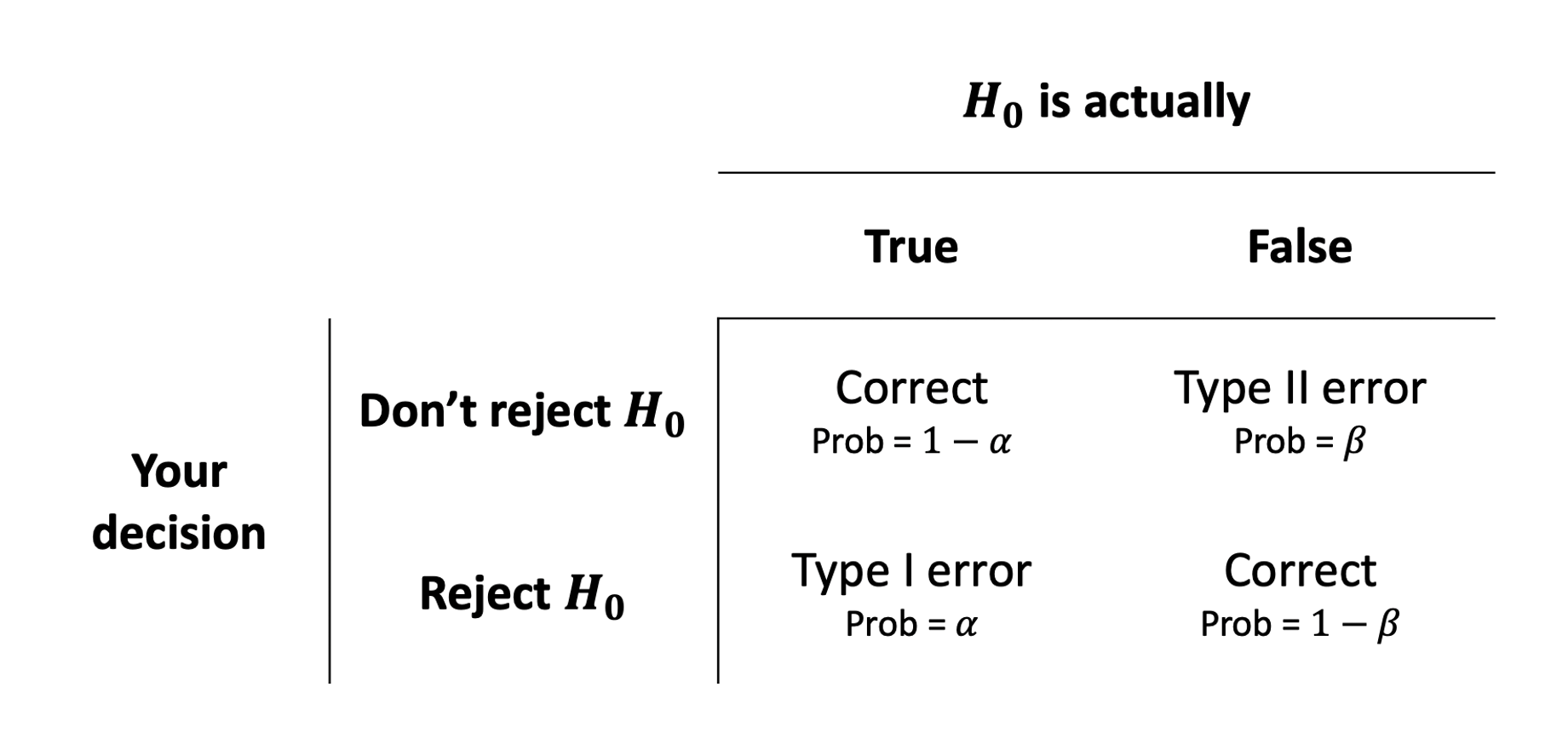
A Type I error corresponds to a false discovery, while a type II error corresponds to a failed discovery/missed opportunity.
Each error has a corresponding probability:
- The probability of incorrectly rejecting a true null hypothesis is \(\alpha = P(\text{Type I error})\)
- The probability of incorrectly not rejecting a false null hypothesis is \(\beta = P(\text{Type II error})\)
A related quantity is Power, which is defined as the probability of correctly rejecting a false null hypothesis.
Power
Power is the probability of rejecting a false null hypothesis. That is, it is the probability that we will find an effect when it is in fact present. \[ \text{Power} = 1 - P(\text{Type II error}) = 1 - \beta \]
See S2 Week 7 lecture, S2 Week 8 lab for further details, examples, and to revise these concepts further.
In practice, it is ideal for studies to have high power while using a relatively small significance level such as .05 or .01. For a fixed \(\alpha\), the power increases in the same cases that P(Type II error) decreases, namely as the sample size increases and as the parameter value moves farther into the H values away from the H0 value.
The power of a test is affected by the following factors:
- sample size. Power increases as the sample size increases.
- effect size. Power increases as the parameter value moves farther into the \(H_1\) values away from the \(H_0\) value.
- significance level. Power increases as the significance level increases.
Out of these, increasing the significance level \(\alpha\) is never an acceptable way to increase power as it leads to more Type I errors, i.e. a higher chance of incorrectly rejecting a true null hypothesis (false discoveries).
As you can see the four quantities above are linked in some complex way, and in this exercises you will see:
How to compute the minimum sample size required to correctly reject a false null hypothesis with a given degree of confidence.
Given sample size constraints, to find what is the probability that you test will correctly reject a false null hypothesis. If it’s too low, you might want to reconsider your study or perhaps even abandon it.
See S2 Week 7 lecture, S2 Week 8 lab for further details, examples, and to revise these concepts further.
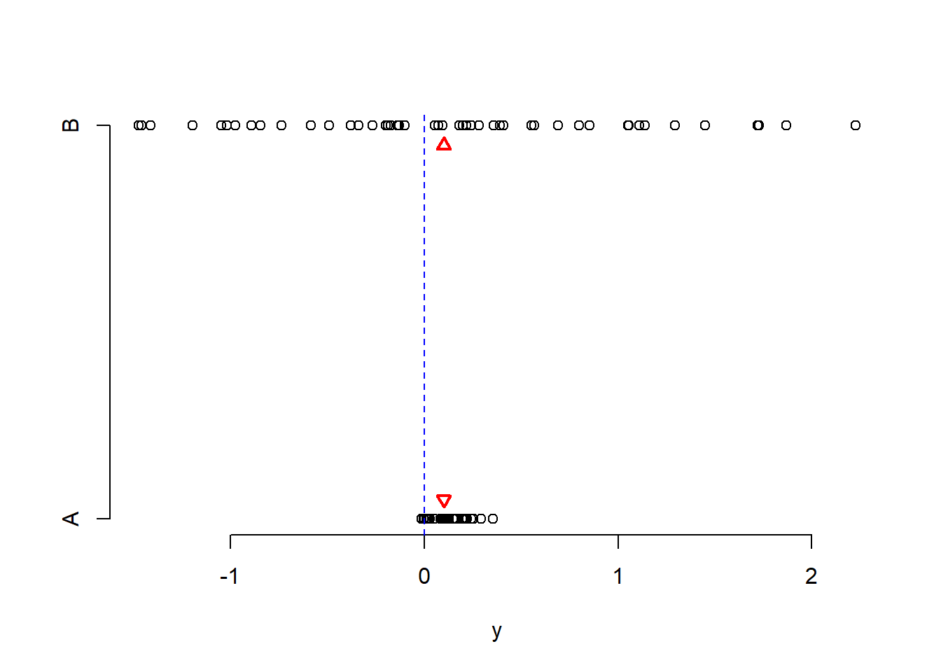
Effect size refers to the “detectability” of your alternative hypothesis. In simple terms, it compares the distance between the alternative and the null hypothesis to the variability in your data.
For simplicity consider comparing a mean: \(H_0: \mu = 0\) vs \(H_1: \mu \neq 0\). If the sample mean were really 0.1 and the null hypothesis is 0, the distance is 0.1 - 0 = 0.1.
Now, a distance of 0.1 has a different weight in the following two scenarios.
Scenario 1. Data vary between -1 and 1.
Scenario 2. Data vary between -1000 and 1000.
Clearly, in Scenario 1 a distance of of 0.1 is a big difference. Conversely, in Scenario 2 a distance of 0.1 is not an interesting difference, it’s negligible compared to the magnitude of the data.
See S2 Week 7 lecture, S2 Week 8 lab for further details, examples, and to revise these concepts further.
You will perform power analysis using the pwr package. To install it, run install.packages("pwr") in your console, then run library(pwr) in your RMarkdown file.
The following functions are available.
| Function | Description |
|---|---|
pwr.2p.test |
Two proportions (equal n) |
pwr.2p2n.test |
Two proportions (unequal n) |
pwr.anova.test |
Balanced one-way ANOVA |
pwr.chisq.test |
Chi-square test |
pwr.f2.test |
General linear model |
pwr.p.test |
Proportion (one sample) |
pwr.r.test |
Correlation |
pwr.t.test |
t-tests (one sample, two samples, paired) |
pwr.t2n.test |
t-test (two samples with unequal n) |
For each function, you can specify three of four arguments (sample size, alpha, effect size, power) and the fourth argument will be calculated for you.
Of the four quantities, effect size is often the most difficult to specify. Calculating effect size typically requires some experience with the measures involved and knowledge of past research.
Typically, specifying effect size requires you to read published literature or past papers on your research topic, to see what effect sizes were found and what significant results were reported. Other times, this might come from previous collected data or subject-knowledge from your colleagues.
But what can you do if you have no clue what effect size to expect in a given study? Cohen (1988) provided guidelines for what a small, medium, or large effect typically is in the behavioral sciences.
| Type of test | Small | Medium | Large | |
|---|---|---|---|---|
| t-test | 0.20 | 0.50 | 0.80 | |
| ANOVA | 0.10 | 0.25 | 0.40 | |
| Linear regression | 0.02 | 0.15 | 0.35 |
See S2 Week 7 lecture, S2 Week 8 lab for further details, examples, and to revise these concepts further.
We compare the mean of a response variable between two groups using a t-test. For example, if you are comparing the mean response between two groups, say treatment and control, the null and alternative hypotheses are: \[ H_0 : \mu_t - \mu_c = 0 \\ H_1 : \mu_t - \mu_c \neq 0 \]
The effect size in this case is Cohen’s \(D\): \[ D = \frac{(\bar x_t - \bar x_c) - 0}{s_p} \] where
- \(\bar x_t\) and \(\bar x_c\) are the sample means in the treatment and control groups, respectively
- \(s_p\) is the “pooled” standard deviation
Cohen’s \(D\) measures the distance between (a) the observed difference in means from (b) the hypothesised value 0, and compares this to the variability in the data.
In R we use the function
pwr.t.test(n = , d = , sig.level = , power = , type = , alternative = )where
-
n= the sample size -
d= the effect size -
sig.level= the significance level \(\alpha\) (the default is 0.05) -
power= the power level. -
type= the type of t-test to perform: either a two-sample t-test (“two.sample”), a one-sample t-test (“one.sample”), or a dependent sample t-test (“paired”). A two-sample test is the default. -
alternative= whether the alternative hypothesis is two-sided (“two.sided”) or one-sided (“less” or “greater”). A two-sided test is the default.
See S2 Week 7 lecture, S2 Week 8 lab for further details, examples, and to revise these concepts further.
In linear regression, the relevant function in R is:
library(pwr)
pwr.f2.test(u = , v = , f2 = , sig.level = , power = )
where - u = numerator degrees of freedom - v = denominator degrees of freedom - f2 = effect size
Here you have one model,
\[ y = \beta_0 + \beta_1 x_1 + \dots + \beta_k x_k + \epsilon \]
and you wish to find the minimum sample size required to answer the following test of hypothesis with a given power:
\[ \begin{aligned} H_0 &: \beta_1 = \beta_2 = \dots = \beta_k = 0 \\ H_1 &: \text{At least one } \beta_i \neq 0 \end{aligned} \]
The appropriate formula for the effect size is:
\[ f^2 = \frac{R^2}{1 - R^2} \]
And the numerator degrees of freedom are \(\texttt u = k\), the number of predictors in the model.
The denominator degrees of freedom returned by the function will give you:
\[ \texttt v = n - (k + 1) = n - k - 1 \]
From which you can infer the sample size as
\[ n = \texttt v + k + 1 \]
In this case you would have a smaller model \(m\) with \(k\) predictors and a larger model \(M\) with \(K\) predictors:
\[ \begin{aligned} m &: \quad y = \beta_0 + \beta_1 x_1 + \dots + \beta_{k} x_k + \epsilon \\ M &: \quad y = \beta_0 + \beta_1 x_1 + \dots + \beta_{k} x_k + \underbrace{\beta_{k + 1} x_{k+1} + \dots + \beta_{K} x_K}_{\text{extra predictors}} + \epsilon \end{aligned} \]
This case is when you wish to find the minimum sample size required to answer the following test of hypothesis:
\[ \begin{aligned} H_0 &: \beta_{k+1} = \beta_{k+2} = \dots = \beta_K = 0 \\ H_1 &: \text{At least one of the above } \beta \neq 0 \end{aligned} \]
You need to use the R-squared from the larger model \(R^2_M\) and the R-squared from the smaller model \(R^2_m\). The appropriate formula for the effect size is:
\[ f^2 = \frac{R^2_{M} - R^2_{m}}{1 - R^2_M} \]
Here, the numerator degrees of freedom are the extra predictors: \(\texttt u = K - k\).
The denominator degrees of freedom returned by the function will give you (here you use \(K\) the number of all predictors in the larger model):
\[ \text v = n - (K + 1) = n - K - 1 \]
From which you can infer the sample size as
\[ n = \text v + K + 1 \]
See S2 Week 7 lecture, S2 Week 8 lab for further details, examples, and to revise these concepts further.
Exploratory analyses are conducted when either (1) you have a hypothesis but no clear analysis plan/strategy; (2) you have lots of variables that might be associated with an outcome variable, but you’re not sure which or in what ways i.e., no clear predictions. It also provides tools for hypothesis generation - particularly via visualisation of data.
Confirmatory analyses are conducted when you have a specific research question to test. You can think of this type of analysis as putting your hypotheses to trial - does your data support or fail to support your argument?
There are a number of steps involved in exploratory analyses:
- Step 1: Check coding of data and visualise variables of interest
- Step 2: Compare models of interest to find if your variables of interest are good predictors of your outcome variable
- Step 3: Compute the k-fold cross validation MSE for each of your models
- Step 4: Identify best fitting model