Effects Coding

Learning Objectives

At the end of this lab, you will:

1. Understand how to specify dummy and sum-to-zero coding
2. Interpret the output from a model using dummy coding
3. Interpret the output from a model using sum-to-zero coding

What You Need

1. Be up to date with lectures
2. Have completed previous lab exercises from Week 1

Required R Packages

Remember to load all packages within a code chunk at the start of your RMarkdown file using library(). If you do not have a package and need to install, do so within the console using install.packages(" "). For further guidance on installing/updating packages, see Section C here.

For this lab, you will need to load the following package(s):

• tidyverse
• psych
• kableExtra

Lab Data

You can download the data required for this lab here or read it in via this link https://uoepsy.github.io/data/RestaurantSpending.csv

Study Overview

Research Question

Does the type of background music playing in a restaurant influence the amount of money that diners spend on their meal?

A group of researchers wanted to test the claims reported in (North, Shilcock, and Hargreaves 2003) on whether the type of background music playing in a restaurant influences the average amount of money spent by diners on their meal.

The group researchers got in touch with a restaurant and asked to alternate silence, popular music, and classical music on successive nights over 18 days. On those nights they recorded the mean spend per head for each table.

Restaurant Spending Codebook

Description

The following variables were collected:

• id: Identifier for each diner
• type: type of music played (“Classical Music”, “Pop Music”, “No Music”)
• amount: restaurant spending per person (in pounds - £)

Preview

The first ten rows of the data are:

id	type	amount
1	No Music	23.14891
2	Pop Music	20.59492
3	Pop Music	19.18172
4	Pop Music	16.70237
5	Classical Music	25.91041
6	Pop Music	19.27888

Setup

Setup

1. Create a new RMarkdown file
2. Load the required package(s)
3. Read the Restaurant Spending dataset into R, assigning it to an object named rest_spend

Solution

#Loading the required package(s)
library(tidyverse)
library(psych)
library(kableExtra)

#Reading in data and storing in object named 'rest_spend'
rest_spend <- read_csv('https://uoepsy.github.io/data/RestaurantSpending.csv')

Exercises

Question 1

Examine the dataset, and perform any necessary and appropriate data management steps.

Solution

Let’s have a look at the data to see what we’re working with:

#first look at dataset structure
str(rest_spend)

spc_tbl_ [360 × 3] (S3: spec_tbl_df/tbl_df/tbl/data.frame)
 $ id    : num [1:360] 1 2 3 4 5 6 7 8 9 10 ...
 $ type  : chr [1:360] "No Music" "Pop Music" "Pop Music" "Pop Music" ...
 $ amount: num [1:360] 23.1 20.6 19.2 16.7 25.9 ...
 - attr(*, "spec")=
  .. cols(
  ..   id = col_double(),
  ..   type = col_character(),
  ..   amount = col_double()
  .. )
 - attr(*, "problems")=<externalptr> 

#now lets look at top 6 rows (or the head) of the dataset
head(rest_spend)

# A tibble: 6 × 3
     id type            amount
  <dbl> <chr>            <dbl>
1     1 No Music          23.1
2     2 Pop Music         20.6
3     3 Pop Music         19.2
4     4 Pop Music         16.7
5     5 Classical Music   25.9
6     6 Pop Music         19.3

Music type is a categorical variable but it is encoded as a character (<chr>) variable rather than a factor (<fctr>). Let’s fix this, and rename ‘type’ to ‘music’ and the levels of the factor to avoid repetition whilst we’re at it:

rest_spend <- rest_spend %>%
    mutate(
        type = factor(type, 
                           levels = c("No Music", "Pop Music", "Classical Music"),
                           labels = c("None", "Pop", "Classical"))) %>%
        rename(music = type)

#re-examine the top 6 rows of the dataset
head(rest_spend)

# A tibble: 6 × 3
     id music     amount
  <dbl> <fct>      <dbl>
1     1 None        23.1
2     2 Pop         20.6
3     3 Pop         19.2
4     4 Pop         16.7
5     5 Classical   25.9
6     6 Pop         19.3

Question 2

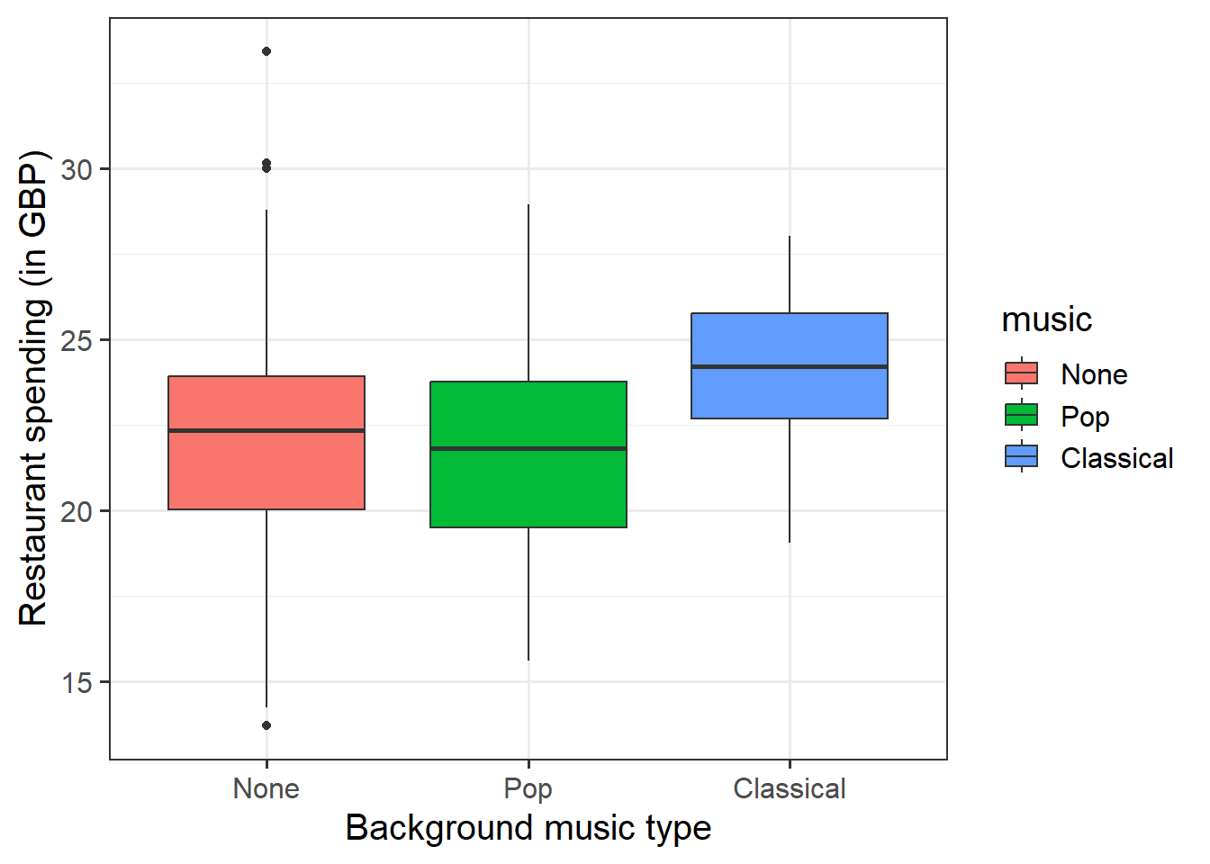
Provide a table of descriptive statistics and visualise your data (remember to interpret your plot in the context of the research question).

Hint

1. For your table of descriptive statistics, both the group_by() and summarise() functions will come in handy here.

2. When visualising the data, consider using geom_boxplot() to visually explore the association between restaurant spending and music type.

3. Make sure to comment on any observed differences among the sample means of the three background music types.

Solution

First, let’s look at our descriptive statistics and present in a well formatted table:

music_desc <- rest_spend %>% 
            group_by(music) %>%
            summarise(n = n(),
                      Mean = mean(amount),
                      SD = sd(amount),
                      Min = min(amount),
                      Max = max(amount)) %>% 
            kable(caption = "Descriptive Statistics", digits = 2) %>%
            kable_styling()

music_desc

Table 1: Descriptive Statistics

music	n	Mean	SD	Min	Max
None	120	22.14	3.44	13.71	33.43
Pop	120	21.90	2.97	15.60	28.94
Classical	120	24.17	1.89	19.05	28.02

Now, let’s visualise the association between restaurant spending and music type using a boxplot:

p1 <- ggplot(data = rest_spend, aes(x = music, y = amount, fill = music)) +
  geom_boxplot() +
  labs(x = 'Background music type', y = 'Restaurant spending (in GBP)')

p1 

Figure 1: Associations among Spending and Music Type

• There are three types of music groups (\(g = 3\)), where there is one group for each music type: “Classical,” “None,” “Pop”. Each group has 120 observations.
• It seems that customers without background music or pop music had a similar average restaurant spending
• The average restaurant spending seems to be higher for those who had a classical music background compared to the customers either without music or with a pop music background.

Dummy Coding

Question 3

Using dummy coding, choose an appropriate reference level to address the research question, and then formally state a linear model to investigate whether there are differences in restaurant spending based on background music conditions.

Describe and schematically represent the coding matrix used in the above model.

Hint

When you reorder the levels, you should end up with the following coding of group means if you choose ‘none’ as your reference group:

• \(\mu_1\) = mean of no music group
• \(\mu_2\) = mean of pop music group
• \(\mu_3\) = mean of classical music group

When schematically representing the coding scheme, you should produce a matrix/table of 0s and 1s.

Solution

It makes sense to have no music as our reference level, since both other groups involve some type of music playing:

#set 'None' music type condition as our reference group. 
rest_spend$music <- fct_relevel(rest_spend$music , "None")

#check the levels of the variable
levels(rest_spend$music)

[1] "None"      "Pop"       "Classical"

Specify our model:

\[ \text{Restaurant Spending} = \beta_0 + \beta_1 \cdot \text{Music(Pop)} + \beta_2 \cdot \text{Music(Classical)} + \epsilon \] In words:

\[ \text{IsPopMusic} = \begin{cases} 1 & \text{if observation is from the Pop Music category} \\ 0 & \text{otherwise} \end{cases} \]

\[ \text{IsClassicalMusic} = \begin{cases} 1 & \text{if observation is from the Classical Music category} \\ 0 & \text{otherwise} \end{cases} \]

Schematically:

\[ \begin{matrix} \textbf{Level} & \textbf{IsPopMusic} & \textbf{IsClassicalMusic} \\ \hline \text{None} & 0 & 0 \\ \text{Pop} & 1 & 0 \\ \text{Clasical} & 0 & 1 \end{matrix} \]

Question 4

Fit the specified model, and assign it the name “mdl_rg” (for reference group constraint).

Interpret your coefficients in the context of the study.

Hint

Under the constraint \(\beta_1 = 0\), meaning that the first factor level is the reference group,

• \(\beta_0\) is interpreted as \(\mu_1\), the mean response for the reference group (group 1);
• \(\beta_i\) is interpreted as the difference between the mean response for group \(i\) and the reference group.

Solution

#fit model
mdl_rg <- lm(amount ~ music, data = rest_spend)

#check output
summary(mdl_rg)

Call:
lm(formula = amount ~ music, data = rest_spend)

Residuals:
   Min     1Q Median     3Q    Max 
-8.433 -1.886  0.127  1.755 11.285 

Coefficients:
               Estimate Std. Error t value Pr(>|t|)    
(Intercept)     22.1414     0.2593  85.373  < 2e-16 ***
musicPop        -0.2424     0.3668  -0.661    0.509    
musicClassical   2.0328     0.3668   5.542 5.81e-08 ***
---
Signif. codes:  0 '***' 0.001 '**' 0.01 '*' 0.05 '.' 0.1 ' ' 1

Residual standard error: 2.841 on 357 degrees of freedom
Multiple R-squared:  0.1151,    Adjusted R-squared:  0.1101 
F-statistic: 23.21 on 2 and 357 DF,  p-value: 3.335e-10

The interpretation is as follows:

Coefficient	Estimate	Corresponds to
(Intercept)	22.1414	\(\hat \beta_0 = \hat \mu_1\)
musicPop	-0.2424	\(\hat \beta_2 = \hat \mu_2 - \hat \beta_0 = \hat \mu_2 - \hat \mu_1\)
musicClassical	2.0328	\(\hat \beta_3 = \hat \mu_3 - \hat \beta_0 = \hat \mu_3 - \hat \mu_1\)

The estimate corresponding to (Intercept) contains \(\hat \beta_0 = \hat \mu_1 = 22.1414\). The estimated average spending for those having no music playing in the background is approximately £22.14.

The next estimate corresponds to musicPop and is \(\hat \beta_1 = -0.2424\). The difference in mean spending between None and Pop is estimated to be \(-0.2424\). In other words, people with pop music playing in the background seem to spend approximately £0.24 less than those who have no music playing in the background.

The estimate corresponding to musicClassical is \(\hat \beta_2 = 2.0328\). This is the estimated difference in mean spending between None and Classical. People with classical music background in the background seem to spend approximately £2.03 more than those who have no music playing in the background.

Hence, for all levels except the reference group we see differences to the reference group while the estimate of the reference level can be found next to (Intercept).

It is also important to notice how the coefficients’ names are written. They are a combination of factor name and level name, such as musicPop. The only coefficient that is missing is musicNone, the one corresponding to the reference category None.

Question 5

Identify the relevant pieces of information from the commands anova(mdl_rg) and summary(mdl_rg) that can be used to conduct an ANOVA \(F\)-test against the null hypothesis that all population means are equal.

Interpret the \(F\)-test results in the context of the ANOVA null hypothesis, and present this output in an APA formatted table.

Hint

To create a table, you can use the kable() function from the kableExtra package here, just like you do for tables of descriptive statistics. Note that we need to list how many digits we want our values to be rounded to in our table: + Degrees of freedom are whole numbers, so 1 will suffice + for all others, we want 2 (in line with APA, but to avoid a \(p\)-value of zero, specify 10

Solution

#examine summary
summary(mdl_rg)

Call:
lm(formula = amount ~ music, data = rest_spend)

Residuals:
   Min     1Q Median     3Q    Max 
-8.433 -1.886  0.127  1.755 11.285 

Coefficients:
               Estimate Std. Error t value Pr(>|t|)    
(Intercept)     22.1414     0.2593  85.373  < 2e-16 ***
musicPop        -0.2424     0.3668  -0.661    0.509    
musicClassical   2.0328     0.3668   5.542 5.81e-08 ***
---
Signif. codes:  0 '***' 0.001 '**' 0.01 '*' 0.05 '.' 0.1 ' ' 1

Residual standard error: 2.841 on 357 degrees of freedom
Multiple R-squared:  0.1151,    Adjusted R-squared:  0.1101 
F-statistic: 23.21 on 2 and 357 DF,  p-value: 3.335e-10

#run anova
anova(mdl_rg)

Analysis of Variance Table

Response: amount
           Df Sum Sq Mean Sq F value    Pr(>F)    
music       2  374.7 187.348  23.211 3.335e-10 ***
Residuals 357 2881.5   8.071                      
---
Signif. codes:  0 '***' 0.001 '**' 0.01 '*' 0.05 '.' 0.1 ' ' 1

The model summary returns the \(F\)-test of model utility which, in this case, corresponds to the ANOVA \(F\)-test against the null hypothesis of equal population means.

The relevant line from summary() is:

F-statistic: 23.21 on 2 and 357 DF,  p-value: 3.335e-10

The relevant parts from anova() are:

• F value of 23.211
• The Df column giving 2 and 357 degrees of freedom
• The p-value of the test, reported under Pr(>F) as 3.335e-10 ***.

We can create a nice table of our anova results:

anova(mdl_rg) %>%
    kable(caption = "Analysis of Variance Table", digits = c(1, 2, 2, 2, 10)) %>%
    kable_styling()

Table 2: Analysis of Variance Table

	Df	Sum Sq	Mean Sq	F value	Pr(>F)
music	2	374.7	187.35	23.21	3e-10
Residuals	357	2881.5	8.07	NA	NA

We can write this up as follows:

We performed an analysis of variance against the null hypothesis of equal population mean spending across three types of background music, \(F(2, 357) = 23.21\), \(p < .001\).

The large observed \(F\)-statistic led to a very small p-value, meaning that such a large observed variability among the mean restaurant spending across the different music types, compared to the variability in the residuals, is very unlikely to happen by chance alone if the population means where all the same (see Table 2).

For this reason, at the 5% significance level, we reject the null hypothesis as there is strong evidence that at least two population means differ.

Question 6

Obtain the estimated (or predicted) group means for the “None,” “Pop,” and “Classical” background music conditions by using the predict() function.

Hint

Step 1: Define a data frame with a column having the same name as the factor in the fitted model (i.e., music). Then, specify all the groups (= levels) for which you would like the predicted mean.

Step 2: Pass the data frame to the predict function using the newdata = argument. The predict() function will match the column named type with the predictor called type in the fitted model ‘mdl_rg’.

See Semester 1 Lab 3 Q8 for a worked example.

Solution

Step 1:

query_groups <- tibble(music = c("None", "Pop", "Classical"))
query_groups

# A tibble: 3 × 1
  music    
  <chr>    
1 None     
2 Pop      
3 Classical

Step 2:

predict(mdl_rg, newdata = query_groups)

       1        2        3 
22.14139 21.89894 24.17414 

• Predicted mean of “None” = \(\hat \mu_\text{None}\) = 22.1414
• Predicted mean of “Pop” = \(\hat \mu_\text{Pop}\) = 22.1414 - 0.2424 = 21.899
• Predicted mean of “Classical” = \(\hat \mu_\text{Classical}\) = 22.1414 + 2.0328 = 24.1742

Sum to Zero Coding

Question 7

Using sum-to-zero coding, formally state a linear model to investigate whether there are differences in restaurant spending based on background music conditions.

Describe and schematically represent the coding matrix used in the above model.

Hint

When schematically representing the coding scheme, you should produce a matrix/table of 0s and 1s.

Solution

Specify our model:

\[ \text{Restaurant Spending} = \beta_0 + \beta_1 \cdot \text{EffectLevel1} + \beta_2 \cdot \text{EffectLevel2} + \epsilon \] In words:

\[ \text{EffectLevel1} = \begin{cases} 1 & \text{if observation is from category 1} \\ 0 & \text{if observation is from category 2} \\ -1 & \text{otherwise} \end{cases} \]

\[ \text{EffectLevel2} = \begin{cases} 0 & \text{if observation is from category 1} \\ 1 & \text{if observation is from category 2} \\ -1 & \text{otherwise} \end{cases} \]

Schematically:

\[ \begin{matrix} \textbf{Level} & \textbf{EffectLevel1} & \textbf{EffectLevel2} \\ \hline \text{None} & 1 & 0 \\ \text{Pop} & 0 & 1 \\ \text{Classical} & -1 & -1 \end{matrix} \]

Question 8

Set the sum to zero constraint for the factor of background music.

Fit again the linear model, and assign the model the name ‘mdl_stz’.

Hint

We can switch between side-constraints using the following code:

#use dummy coding
contrasts(rest_spend$music) <- "contr.treatment"

#use sum-to-zero coding
contrasts(rest_spend$music) <- "contr.sum"

Solution

contrasts(rest_spend$music) <- "contr.sum"

#check coding matches our table above:
contrasts(rest_spend$music)

          [,1] [,2]
None         1    0
Pop          0    1
Classical   -1   -1

mdl_stz <- lm(amount ~ music, data = rest_spend)
summary(mdl_stz)

Call:
lm(formula = amount ~ music, data = rest_spend)

Residuals:
   Min     1Q Median     3Q    Max 
-8.433 -1.886  0.127  1.755 11.285 

Coefficients:
            Estimate Std. Error t value Pr(>|t|)    
(Intercept)  22.7382     0.1497 151.856  < 2e-16 ***
music1       -0.5968     0.2118  -2.818   0.0051 ** 
music2       -0.8392     0.2118  -3.963 8.94e-05 ***
---
Signif. codes:  0 '***' 0.001 '**' 0.01 '*' 0.05 '.' 0.1 ' ' 1

Residual standard error: 2.841 on 357 degrees of freedom
Multiple R-squared:  0.1151,    Adjusted R-squared:  0.1101 
F-statistic: 23.21 on 2 and 357 DF,  p-value: 3.335e-10

Question 9

Interpret your coefficients in the context of the study.

Hint

Recall that under this constraint the interpretation of the coefficients becomes:

• \(\beta_0\) represents the grand mean
• \(\beta_i\) the effect due to group \(i\) — that is, the mean response in group \(i\) minus the grand mean

Solution

The interpretation is as follows:

Coefficient	Estimate	Corresponds to
(Intercept)	22.7382	\(\beta_0 = \frac{\mu_1 + \mu_2 + \mu_3}{3} = \mu\)
music1	-0.5968	\(\beta_1 = \mu_1 - \mu\)
music2	-0.8392	\(\beta_2 = \mu_2 - \mu\)

The estimate corresponding to (Intercept) contains \(\beta_0 = \mu = 22.7382\). This value represents the grand mean of the data. The estimated average spending for customers across background music conditions is approximately £22.74.

The next estimate corresponds to music1 and is \(\hat \beta_1 = -0.5968\). The difference in mean spending between None and the grand mean is estimated to be \(-0.5968\). In other words, people with no music playing in the background seem to spend approximately £0.60 less than average.

The estimate corresponding to music2 is \(\hat \beta_2 = -0.8392\). The difference in mean spending between Pop and the grand mean is estimated to be \(-0.8392\). In other words, customers with Pop music playing in the background seem to spend approximately £0.84 less than average.

The estimate for music3, representing the difference of “Classical” to the grand mean is not shown by summary(). Because of the side-constraint, we know it must be \(\beta_3 = -(\beta_1 + \beta_2)\). The difference in mean spending between Classical and the grand mean is estimated to be \(-(-0.5968 + -0.8392) = 1.436\). In other words, customers with Classical music playing in the background seem to spend approximately £1.44 more than average.

Comparing Approaches

Question 10

Compare the the predicted group means across both contrast approaches - do they match?

Is the model utility \(F\)-test still the same across both approaches? Why do you think it’s the case?

Solution

#note that the below two models and dataset have already been created above, so you can jump straight to adding the predicted values from the two models if you'd prefer 

#model with dummy coding
contrasts(rest_spend$music) <- contr.treatment
mdl_rg <- lm(amount ~ music, data = rest_spend)

# model with sum-to-zero coding
contrasts(rest_spend$music) <- contr.sum
mdl_stz <- lm(amount ~ music, data = rest_spend)

#create dataset
music_groups <- tibble(music = c("None", "Pop", "Classical"))
music_groups

# A tibble: 3 × 1
  music    
  <chr>    
1 None     
2 Pop      
3 Classical

#add predicted values from our two models - mdl_rg & mdl_stz - values are the same
music_groups %>%
  mutate(
    pred_dummy = predict(mdl_rg, newdata = .),
    pred_sum_to_zero = predict(mdl_stz, newdata = .)
  )

# A tibble: 3 × 3
  music     pred_dummy pred_sum_to_zero
  <chr>          <dbl>            <dbl>
1 None            22.1             22.1
2 Pop             21.9             21.9
3 Classical       24.2             24.2

#compare anova() outputs - values are the same
anova(mdl_rg)

Analysis of Variance Table

Response: amount
           Df Sum Sq Mean Sq F value    Pr(>F)    
music       2  374.7 187.348  23.211 3.335e-10 ***
Residuals 357 2881.5   8.071                      
---
Signif. codes:  0 '***' 0.001 '**' 0.01 '*' 0.05 '.' 0.1 ' ' 1

anova(mdl_stz)

Analysis of Variance Table

Response: amount
           Df Sum Sq Mean Sq F value    Pr(>F)    
music       2  374.7 187.348  23.211 3.335e-10 ***
Residuals 357 2881.5   8.071                      
---
Signif. codes:  0 '***' 0.001 '**' 0.01 '*' 0.05 '.' 0.1 ' ' 1

Yes, the values from both the dummy coding and sum-to-zero approaches give the same values. This is because, regardless of the coding matrix scheme we use to compare groups, we are still modelling the same group means from our data set. Thus, neither the predicted means nor the model utility \(F\)-test depend on the side-constraint that we employ. However, the side-constraint affects the meaning of the parameters in the model.

References

North, A., A. Shilcock, and D. Hargreaves. 2003. “The Effect of Musical Style on Restaurant Customers’ Spending.” Environment and Behavior 35: 712–18.