Model Comparisons

Learning Objectives

At the end of this lab, you will:

1. Understand measures of model fit using F.
   
2. Understand the principles of model selection and how to compare models via F tests.
3. Understand AIC and BIC.

What You Need

1. Be up to date with lectures
2. Have completed previous lab exercises from Semester 1

Required R Packages

Remember to load all packages within a code chunk at the start of your RMarkdown file using library(). If you do not have a package and need to install, do so within the console using install.packages(" "). For further guidance on installing/updating packages, see Section C here.

For this lab, you will need to load the following package(s):

• tidyverse
• stargazer

Lab Data

You can download the data required for this lab here or read it in via this link https://uoepsy.github.io/data/wellbeing_rural.csv

Study Overview

Research Questions

• RQ1: Is there an overall effect of the number of social interactions on wellbeing scores?
• RQ2: Does the association between number of social interactions and wellbeing differ between rural and non-rural residents?
• RQ3: Does weekly outdoor time explain a significant amount of variance in wellbeing scores over and above the interaction between weekly social interactions and location (rural vs not-rural)?

Wellbeing/Rurality data codebook.

Description

From the Edinburgh & Lothians, 100 city/suburb residences and 100 rural residences were chosen at random and contacted to participate in the study. The Warwick-Edinburgh Mental Wellbeing Scale (WEMWBS), was used to measure mental health and well-being.

Participants filled out a questionnaire including items concerning: estimated average number of hours spent outdoors each week, estimated average number of social interactions each week (whether on-line or in-person), whether a daily routine is followed (yes/no). For those respondents who had an activity tracker app or smart watch, they were asked to provide their average weekly number of steps.

The data in wellbeing.csv contain seven attributes collected from a random sample of \(n=200\) hypothetical residents over Edinburgh & Lothians, and include:

• wellbeing: Warwick-Edinburgh Mental Wellbeing Scale (WEMWBS), a self-report measure of mental health and well-being. The scale is scored by summing responses to each item, with items answered on a 1 to 5 Likert scale. The minimum scale score is 14 and the maximum is 70.
  
• outdoor_time: Self report estimated number of hours per week spent outdoors
  
• social_int: Self report estimated number of social interactions per week (both online and in-person)
• routine: Binary 1=Yes/0=No response to the question “Do you follow a daily routine throughout the week?”
• location: Location of primary residence (City, Suburb, Rural)
• steps_k: Average weekly number of steps in thousands (as given by activity tracker if available)
• age: Age in years of respondent

Preview

The first six rows of the data are:

age	outdoor_time	social_int	routine	wellbeing	location	steps_k
28	12	13	1	36	rural	21.6
56	5	15	1	41	rural	12.3
25	19	11	1	35	rural	49.8
60	25	15	0	35	rural	NA
19	9	18	1	32	rural	48.1
34	18	13	1	34	rural	67.3

Setup

Setup

1. Create a new RMarkdown file
2. Load the required package(s)
3. Read the wellbeing_rural dataset into R, assigning it to an object named wrdata

Solution

#Loading the required package(s)
library(tidyverse)
library(stargazer)

#Reading in data and storing in object named 'wrdata'
wrdata <- read_csv("https://uoepsy.github.io/data/wellbeing_rural.csv")

Exercises

Question 1

Check coding of variables (e.g., that categorical variables are coded as factors), and create a new binary variable which specifies whether or not each participant lives in a rural location.

Hint

You will need to use two functions - firstly mutate(), and then ifelse() when creating your new variable (which should also be coded as a factor).

Solution

#before we create our new variable, it would be helpful to give a more informative name to the levels of the routine variable as opposed to 0s and 1s

wrdata <-  wrdata %>% 
    mutate(
        routine = factor(routine,
                         levels = c(0,1),
                         labels = c("No", "Yes")),
        isRural = factor(ifelse(location == "rural","rural","not rural"))
    )

Question 2

Using fct_relevel(), specify ‘not rural’ as your reference group for your newly created variable (i.e., the isRural variable).

Solution

wrdata$isRural <- fct_relevel(wrdata$isRural, "not rural")

Question 3

Fit the below 5 models required to address the three research questions stated above. Note down which model(s) will be used to address each research question, and examine the results of each model.

Name the models as follows: “wb_mdl0”, “wb_mdl1”, “wb_mdl2”, “wb_mdl3”, and “wb_mdl4”.

\[ \text{Wellbeing} = \beta_0 + \epsilon \]
\[ \text{Wellbeing} = \beta_0 + \beta_1 \cdot Social Interactions + \epsilon \]
\[ \text{Wellbeing} = \beta_0 + \beta_1 \cdot Social Interactions + \beta_2 \cdot Location_{Rural} + \epsilon \]
\[ \begin{split} \text{Wellbeing} = \beta_0 + \beta_1 \cdot Social Interactions + \beta_2 \cdot Location_{Rural} \\+ \beta_3 \cdot (Social Interactions \cdot Location_{Rural}) + \epsilon \end{split} \]
\[ \begin{split} \text{Wellbeing} = \beta_0 + \beta_1 \cdot Social Interactions + \beta_2 \cdot Location_{Rural} \\+ \beta_3 \cdot (Social Interactions \cdot Location_{Rural}) + \beta_4 \cdot \text{Outdoor Time} + \epsilon \end{split} \]

Hint

The summary() function will be useful to examine the model output.

Solution

#null/intercept only model
wb_mdl0 <- lm(wellbeing ~ 1, data = wrdata)
summary(wb_mdl0)

Call:
lm(formula = wellbeing ~ 1, data = wrdata)

Residuals:
    Min      1Q  Median      3Q     Max 
-14.295  -3.295  -1.295   3.705  22.705 

Coefficients:
            Estimate Std. Error t value Pr(>|t|)    
(Intercept)  36.2950     0.3813   95.19   <2e-16 ***
---
Signif. codes:  0 '***' 0.001 '**' 0.01 '*' 0.05 '.' 0.1 ' ' 1

Residual standard error: 5.392 on 199 degrees of freedom

#model with social interactions
wb_mdl1 <- lm(wellbeing ~ social_int, data = wrdata)
summary(wb_mdl1)

Call:
lm(formula = wellbeing ~ social_int, data = wrdata)

Residuals:
     Min       1Q   Median       3Q      Max 
-15.5628  -3.2741  -0.7908   3.3703  20.4706 

Coefficients:
            Estimate Std. Error t value Pr(>|t|)    
(Intercept) 32.40771    1.17532  27.573  < 2e-16 ***
social_int   0.32220    0.09243   3.486 0.000605 ***
---
Signif. codes:  0 '***' 0.001 '**' 0.01 '*' 0.05 '.' 0.1 ' ' 1

Residual standard error: 5.247 on 198 degrees of freedom
Multiple R-squared:  0.05781,   Adjusted R-squared:  0.05306 
F-statistic: 12.15 on 1 and 198 DF,  p-value: 0.0006045

#model with social interactions and location (rural vs non-rural)
wb_mdl2 <- lm(wellbeing ~ social_int + isRural, data = wrdata)
summary(wb_mdl2)

Call:
lm(formula = wellbeing ~ social_int + isRural, data = wrdata)

Residuals:
     Min       1Q   Median       3Q      Max 
-13.3711  -3.1794   0.1097   2.5407  17.6324 

Coefficients:
             Estimate Std. Error t value Pr(>|t|)    
(Intercept)  34.11591    1.07052  31.868  < 2e-16 ***
social_int    0.38167    0.08257   4.622 6.85e-06 ***
isRuralrural -4.85152    0.66283  -7.319 6.18e-12 ***
---
Signif. codes:  0 '***' 0.001 '**' 0.01 '*' 0.05 '.' 0.1 ' ' 1

Residual standard error: 4.664 on 197 degrees of freedom
Multiple R-squared:  0.2593,    Adjusted R-squared:  0.2517 
F-statistic: 34.47 on 2 and 197 DF,  p-value: 1.453e-13

#model with social interactions and location (rural vs non-rural) interaction term
wb_mdl3 <- lm(wellbeing ~ social_int*isRural, data = wrdata)
summary(wb_mdl3)

Call:
lm(formula = wellbeing ~ social_int * isRural, data = wrdata)

Residuals:
     Min       1Q   Median       3Q      Max 
-12.4845  -2.7975   0.0155   2.4539  15.6743 

Coefficients:
                        Estimate Std. Error t value Pr(>|t|)    
(Intercept)              30.9986     1.4284  21.702  < 2e-16 ***
social_int                0.6488     0.1160   5.593 7.42e-08 ***
isRuralrural              1.3866     2.0510   0.676  0.49981    
social_int:isRuralrural  -0.5176     0.1615  -3.206  0.00157 ** 
---
Signif. codes:  0 '***' 0.001 '**' 0.01 '*' 0.05 '.' 0.1 ' ' 1

Residual standard error: 4.558 on 196 degrees of freedom
Multiple R-squared:  0.2962,    Adjusted R-squared:  0.2854 
F-statistic: 27.49 on 3 and 196 DF,  p-value: 6.97e-15

#model with social interactions and location (rural vs non-rural) term, and outdoor time
wb_mdl4 <- lm(wellbeing ~ social_int*isRural + outdoor_time, data= wrdata)
summary(wb_mdl4)

Call:
lm(formula = wellbeing ~ social_int * isRural + outdoor_time, 
    data = wrdata)

Residuals:
     Min       1Q   Median       3Q      Max 
-12.7426  -2.6884  -0.1465   2.7122  14.3407 

Coefficients:
                        Estimate Std. Error t value Pr(>|t|)    
(Intercept)             27.61305    1.61227  17.127  < 2e-16 ***
social_int               0.65490    0.11175   5.861 1.94e-08 ***
isRuralrural             1.46796    1.97579   0.743   0.4584    
outdoor_time             0.17704    0.04395   4.028 8.04e-05 ***
social_int:isRuralrural -0.51129    0.15554  -3.287   0.0012 ** 
---
Signif. codes:  0 '***' 0.001 '**' 0.01 '*' 0.05 '.' 0.1 ' ' 1

Residual standard error: 4.391 on 195 degrees of freedom
Multiple R-squared:  0.3502,    Adjusted R-squared:  0.3369 
F-statistic: 26.28 on 4 and 195 DF,  p-value: < 2.2e-16

The models required to address each research question (RQ) are as follows:

• RQ1: Models wb_mdl0 and wb_mdl1
• RQ2: Models wb_mdl2 and wb_mdl3
• RQ3: Models wb_mdl3 and wb_mdl4

Question 4

Provide key model results from the two models required to address RQ1 - whether there is an overall effect of the number of social interactions on wellbeing scores - in a single formatted table.

Hint

You will need to use a new package to do this - stargazer.

Like tab_model() that you have used in many previous labs, stargazer() can take lots of different arguments to customize and build a table. You may want to consider specifying the below (and remember you can use the helper function via ?stargazer() for further information about the functionality of the package):

• title = - specify the title of your table
• dep.var.labels = - specify the name of your dependent variable(s)
• covariate.labels = - specify the names of your covariates (or independent) variables
• type = - specify whether you want ‘html’ (use when knitting to HTML), ‘latex’ (use when knitting to PDF), or ‘text’ (use when knitting to Word)
• digits = - specify rounding (remember APA standard is, in most cases, 2 decimal places)
• intercept.bottom = - specify if you want the intercept (or ‘constant’) value to be printed at the bottom (TRUE) or top (FALSE) of the output

Note

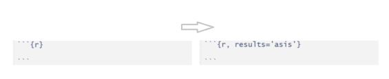
Your table will only render once you have knitted your document. Within your code chunk options, you may need to specify results = 'asis'.

You can learn more about updating your code chunk options here, and you should end up with the below:

Solution

stargazer(wb_mdl0, wb_mdl1,
          title="Regression Model Results for RQ1",
          dep.var.labels=c("Wellbeing Score"),
          covariate.labels=c("Intercept", "Number of Social Interactions"), 
          type = "html", 
          digits = 2,
          single.row=TRUE, 
          align=TRUE,
          intercept.bottom = FALSE)

Regression Model Results for RQ1

	Dependent variable:
	Wellbeing Score
	(1)	(2)
Intercept	36.29*** (0.38)	32.41*** (1.18)
Number of Social Interactions		0.32*** (0.09)
Observations	200	200
R2	0.00	0.06
Adjusted R2	0.00	0.05
Residual Std. Error	5.39 (df = 199)	5.25 (df = 198)
F Statistic		12.15*** (df = 1; 198)
Note:	p<0.1; p<0.05; p<0.01

Question 5

Is there a main effect of the number of weekly social interactions?

Check that the \(F\)-statistic and the \(p\)-value are the the same as that which is given at the bottom of summary(wb_mdl1).

Hint

Use the anova() function to perform a model comparison between your model with social interactions (wb_mdl1) to the null model (wb_mdl0).

Remember that the null model tests the null hypothesis that all beta coefficients are zero. By comparing wb_mdl0 to wb_mdl1, we can test whether we should include the IV of social_int.

Solution

# model comparison wb_mdl0 vs wb_mdl1
anova(wb_mdl0, wb_mdl1)

Analysis of Variance Table

Model 1: wellbeing ~ 1
Model 2: wellbeing ~ social_int
  Res.Df    RSS Df Sum of Sq     F    Pr(>F)    
1    199 5785.6                                 
2    198 5451.1  1    334.49 12.15 0.0006045 ***
---
Signif. codes:  0 '***' 0.001 '**' 0.01 '*' 0.05 '.' 0.1 ' ' 1

# extract f statistic from summary of wb_mdl1
summary(wb_mdl1)$fstatistic

    value     numdf     dendf 
 12.14975   1.00000 198.00000 

# we can retrieve the p-value:
fstat = summary(wb_mdl1)$fstatistic[1]
df_1 = summary(wb_mdl1)$fstatistic[2]
df_2 = summary(wb_mdl1)$fstatistic[3]
pf(fstat, df_1, df_2, lower.tail = FALSE)

       value 
0.0006045334 

The number of social interactions was found to explain a significant amount of variance in wellbeing scores (\(F\)(1 )=12.15, \(p\)<.001). There was a main effect of social interactions.

Question 6

Does the association between number of social interactions and wellbeing differ between rural and non-rural residents?

Provide key model results from the two models in a single formatted table, and report the results of the model comparison in APA format.

Hint

To address RQ2, you need to compare “wb_mdl2” and “wb_mdl3”

Solution

stargazer(wb_mdl2, wb_mdl3,
          title="Regression Model Results for RQ2",
          dep.var.labels=c("Wellbeing Score"),
          covariate.labels=c("Intercept", "Number of Social Interactions", "Location - Rural", "Number of Social Interactions * Location - Rural"), 
          type = "html", 
          digits = 2,
          single.row=TRUE, 
          align=TRUE,
          intercept.bottom = FALSE)

Regression Model Results for RQ2

	Dependent variable:
	Wellbeing Score
	(1)	(2)
Intercept	34.12*** (1.07)	31.00*** (1.43)
Number of Social Interactions	0.38*** (0.08)	0.65*** (0.12)
Location - Rural	-4.85*** (0.66)	1.39 (2.05)
Number of Social Interactions * Location - Rural		-0.52*** (0.16)
Observations	200	200
R2	0.26	0.30
Adjusted R2	0.25	0.29
Residual Std. Error	4.66 (df = 197)	4.56 (df = 196)
F Statistic	34.47*** (df = 2; 197)	27.49*** (df = 3; 196)
Note:	p<0.1; p<0.05; p<0.01

# model comparison wb_mdl0 vs wb_mdl1
anova(wb_mdl2, wb_mdl3)

Analysis of Variance Table

Model 1: wellbeing ~ social_int + isRural
Model 2: wellbeing ~ social_int * isRural
  Res.Df    RSS Df Sum of Sq      F   Pr(>F)   
1    197 4285.6                                
2    196 4072.1  1    213.49 10.276 0.001574 **
---
Signif. codes:  0 '***' 0.001 '**' 0.01 '*' 0.05 '.' 0.1 ' ' 1

There was a significant interaction between the number of social interactions and location (rural vs non-rural) (\(F\)(1 )=10.28, \(p\)<.001). This suggested that the association between number of social interactions and wellbeing did differ between rural and non-rural residents.

Question 7

Look at the amount of variation in wellbeing scores explained by models “wb_mdl3” and “wb_mdl4”.

From this, can we answer the third research question of whether weekly outdoor time explains a significant amount of variance in wellbeing scores over and above the interaction between weekly social interactions and location (rural vs not-rural)?

Provide justification/rationale for your answer.

Hint

Recall from Semester 1 that to determine how much variation is explained by a model, we need to look at our \(R^2\) values (specifically the adjusted \(R^2\) value in this case since the models have multiple predictors.

Solution

Let’s look at the amount of variance explained by each model:

summary(wb_mdl3)$adj.r.squared

[1] 0.2853841

summary(wb_mdl4)$adj.r.squared

[1] 0.3369022

The model with weekly outdoor time as a predictor explains 34% of the variance, and the model without explains 29%. But, from only looking at the proportion of variance accounted for in each model, we cannot determine which model is statistically a better fit. To answer the question ‘Does including weekly outdoor time as a predictor provide a significantly better fit of the data?’ we need to statistically compare wb_mdl3 to wb_mdl4.

Question 8

Does weekly outdoor time explain a significant amount of variance in wellbeing scores over and above the interaction between weekly social interactions and location (rural vs not-rural)?

Provide key model results from the two models in a single formatted table, and report the results of the model comparison in APA format.

Hint

To address RQ3, you need to compare “wb_mdl3” and “wb_mdl4”

Solution

stargazer(wb_mdl3, wb_mdl4,
          title="Regression Model Results for RQ3",
          dep.var.labels=c("Wellbeing Score"),
          covariate.labels=c("Intercept", "Number of Social Interactions", "Location - Rural", "Outdoor Time (Hours)", "Number of Social Interactions * Location - Rural"), 
          type = "html", 
          digits = 2,
          single.row=TRUE, 
          align=TRUE,
          intercept.bottom = FALSE)

Regression Model Results for RQ3

	Dependent variable:
	Wellbeing Score
	(1)	(2)
Intercept	31.00*** (1.43)	27.61*** (1.61)
Number of Social Interactions	0.65*** (0.12)	0.65*** (0.11)
Location - Rural	1.39 (2.05)	1.47 (1.98)
Outdoor Time (Hours)		0.18*** (0.04)
Number of Social Interactions * Location - Rural	-0.52*** (0.16)	-0.51*** (0.16)
Observations	200	200
R2	0.30	0.35
Adjusted R2	0.29	0.34
Residual Std. Error	4.56 (df = 196)	4.39 (df = 195)
F Statistic	27.49*** (df = 3; 196)	26.28*** (df = 4; 195)
Note:	p<0.1; p<0.05; p<0.01

anova(wb_mdl3, wb_mdl4)

Analysis of Variance Table

Model 1: wellbeing ~ social_int * isRural
Model 2: wellbeing ~ social_int * isRural + outdoor_time
  Res.Df    RSS Df Sum of Sq      F    Pr(>F)    
1    196 4072.1                                  
2    195 3759.3  1    312.85 16.228 8.043e-05 ***
---
Signif. codes:  0 '***' 0.001 '**' 0.01 '*' 0.05 '.' 0.1 ' ' 1

Weekly outdoor time was found to explain a significant amount of variance in wellbeing scores over and above weekly social interactions and location (\(F\)(1 )=16.23, \(p\)<.001).

Question 9

Compare the two following models, each looking at the associations of Wellbeing scores and two different predictor variables.

\(\text{Wellbeing} = \beta_0 + \beta_1 \cdot \text{Social Interactions} + \beta_2 \cdot \text{Age} + \epsilon\)

\(\text{Wellbeing} = \beta_0 + \beta_1 \cdot \text{Outdoor Time} + \beta_2 \cdot \text{Routine} + \epsilon\)

In APA format, report which model you think best fits the data.

Hint

Compare using AIC() and BIC() since the models are non-nested.

Solution

#fit models
wb_socint_age <- lm(wellbeing ~ social_int + age, data = wrdata)
wb_outdoor_routine <- lm(wellbeing ~ outdoor_time + routine, data = wrdata)

#AIC values
AIC(wb_socint_age, wb_outdoor_routine)

                   df      AIC
wb_socint_age       4 1236.575
wb_outdoor_routine  4 1220.914

#BIC values
BIC(wb_socint_age, wb_outdoor_routine)

                   df      BIC
wb_socint_age       4 1249.769
wb_outdoor_routine  4 1234.108

We used AIC and BIC model selection to distinguish between two possible models describing the association between several personal factors and wellbeing scores. The model with outdoor time and routine included as predictors was better fitting (AIC = 1220.91) the alternative model with weekly number of social interactions and age (AIC = 1236.58). Based on the BIC value of the former model (BIC = 1234.11) we concluded that it was substantively better fitting than the alternative, latter model (BIC = 1249.77).

Question 10

The code below fits 5 different models based on our wrdata:

model1 <- lm(wellbeing ~ social_int + outdoor_time, data = wrdata)
model2 <- lm(wellbeing ~ social_int + outdoor_time + age, data = wrdata)
model3 <- lm(wellbeing ~ social_int + outdoor_time + routine, data = wrdata)
model4 <- lm(wellbeing ~ social_int + outdoor_time + routine + age, data = wrdata)
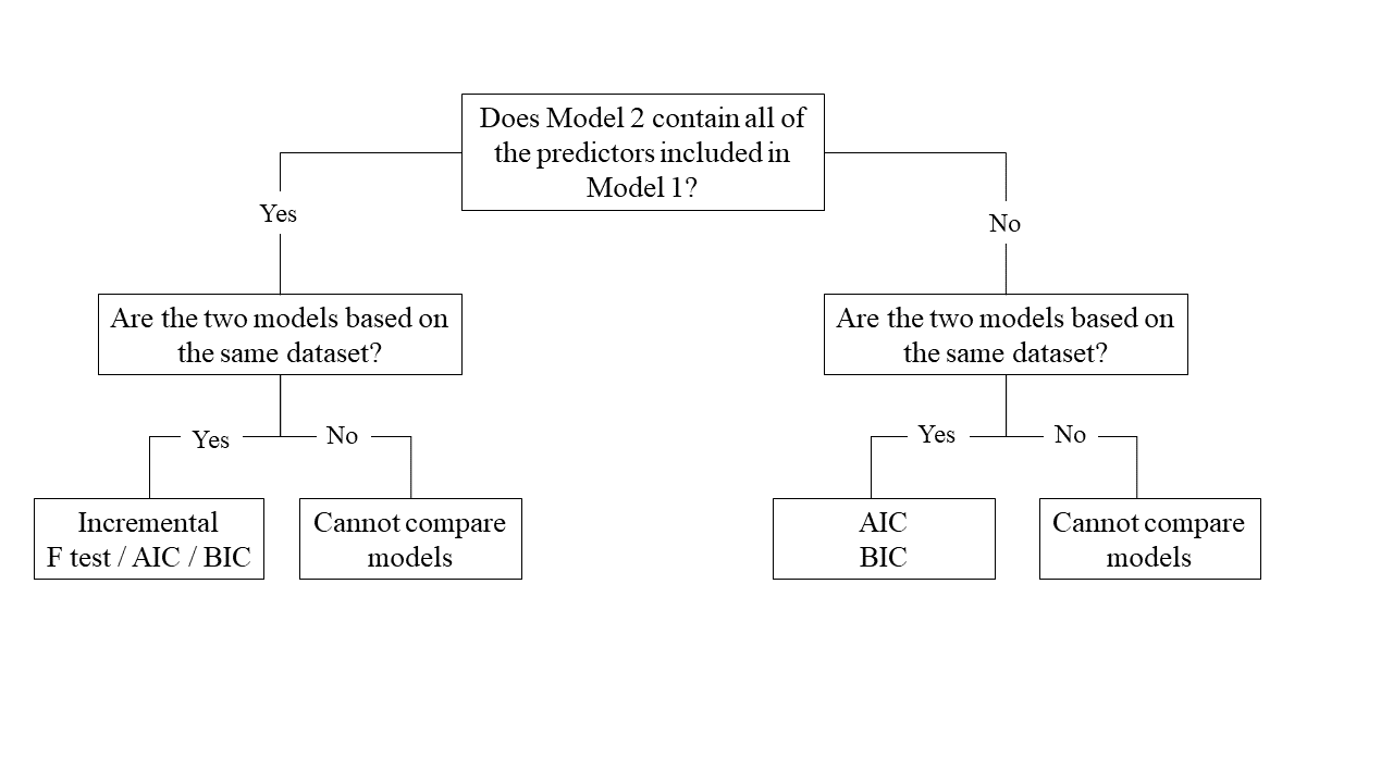
model5 <- lm(wellbeing ~ social_int + outdoor_time + routine + steps_k, data = wrdata)

For each of the below pairs of models, what methods are/are not available for us to use for comparison and why?

• model1 vs model2
• model2 vs model3
• model1 vs model4
• model3 vs model5

This flowchart might help you to reach your decision:

Hint

You may need to examine the dataset, and check for accuracy (e.g., are there any impossible / out of range values?) and completeness (e.g., are there any missing values?).

Solution

• model1 vs model2
  These models are nested - model2 contains all the variables of model1 and they are fitted on the same dataset.
  We can therefore use an \(F\)-test or AIC and BIC.

• model2 vs model3
  These models are not nested, but they are fitted on the same dataset.
  We can therefore use AIC or BIC, but we cannot use an \(F\)-test.

• model1 vs model4 These models are nested - model4 contains all the variables of model1 and they are fitted on the same dataset.
  We can therefore use an \(F\)-test or AIC and BIC.

• model3 vs model5
  These models are not nested, and they are not fitted on the same dataset. The “steps_k” variable contains missing values (over 30% of the data is missing for this variable), and so these whole rows are excluded from model5 (but they are included in model3). We cannot compare these models.