Functions and Models

Learning Objectives

At the end of this lab, you will:

1. Have reviewed the main concepts from introductory statistics.
2. Understand the concept of a function.
3. Be able to discuss what a statistical model is.
4. Understand the link between models and functions.

Requirements

1. Have attended and/or watched Week 1 lectures.
2. Have installed R and RStudio on your own computer (unless you have a Chromebook where you may continue to use the PPLS RStudio Server).

Required R Packages

Remember to load all packages within a code chunk at the start of your RMarkdown file using library(). If you do not have a package and need to install, do so within the console using install.packages(" "). For further guidance on installing/updating packages, see Section C here.

For this lab, you will need to load the following package(s):

• tidyverse
• ggExtra
• kableExtra

Lab Data

You can download the data required for this lab here or read it in via this link https://uoepsy.github.io/data/handheight.csv.

Setup

Setup

1. Create a new RMarkdown file
2. Load the required package(s)
3. Read the handheight dataset into R, assigning it to an object named handheight

Solution

#Loading the required package(s)
library(tidyverse)
library(ggExtra)
library(kableExtra)

# Reading in data and storing to an object named 'handheight'
handheight <- read_csv('https://uoepsy.github.io/data/handheight.csv')

Refresher of Basic Terminology

Question 1

Provide a short definition for each of these terms.

• (Observational) unit
• Variable
• Categorical variable
• Numeric variable
• Response/dependent variable
• Explanatory/independent variable
• Observational study
• Experiment

Check the flashcards in the solution below to compare your definition. If you are not comfortable with one (or more) of the terms, revisit the DAPR1 materials for a refresher.

Solution

(Observational) unit

The individual entities on which data are collected.

Variable

Any characteristic recorded on the observational units.

Categorical variable

A categorical variable places units into one of several groups. Examples are country of birth, dominant hand, and eye colour.

Numeric variable

A variable that records a numerical quantity for each case. For such variables standard arithmetic operations make sense. For example, average height, IQ, and weight.

Response/dependent variable

A response variable (also called a dependent variable) measures the outcome of interest in a study.

Explanatory/independent variable

Explanatory variables (also called independent variables or predictors) are used to explain changes in the response variable.

Observational study

An observational study is a study in which the researcher does not manipulate any of the variables involved in the study, but merely records the values as they naturally exist.

Experiment

An experiment is a study in which the researcher imposes the values of the explanatory variable on the units before measuring the response variable.

Functions and Mathematical Models

Question 2

Consider the function \(y = 2 + 5 \ x\).

• Identify the dependent variable (DV)
• Identify the independent variable (IV)
• Describe in words what the function does, and compute the output for the following input:

\[ x = \begin{bmatrix} 2 \\ 6 \end{bmatrix} \]

Solution

The function says that the \(y\) value is obtained as a transformation of the \(x\) value.

• The dependent variable is \(y\)
• The independent variable is \(x\)
• The \(y\) value is obtained as five times \(x\), plus two.

Example (1): If \(x\) equals 2, the corresponding value of \(y\) will be \(2 + 5 * 2 = 12\).
Example (2): If \(x\) equals 6, the corresponding value of \(y\) will be \(2 + 5 * 6 = 32\). \[ y = \begin{bmatrix} 2 + 5 * 2 \\ 2 + 5 * 6 \end{bmatrix} = \begin{bmatrix} 12 \\ 32 \end{bmatrix} \]

Question 3

Write down in words and in symbols the function describing the relationship between the side of a square and its perimeter.

Hint

We are interested in how the perimeter varies as a function of its side. Hence, the perimeter is the dependent variable, and the side is the independent variable.

Solution

In words:

The perimeter of a square is four times the length of its side.

In symbols:

The relationship between side and perimeter of squares is given by: \[ Perimeter = 4 * Side \]

If you denote \(y\) as the dependent variable Perimeter, and \(x\) as the independent variable Side we cam write rewrite as: \[ y = 4 * x \]

Functions and Mathematical Models: Plots

Question 4

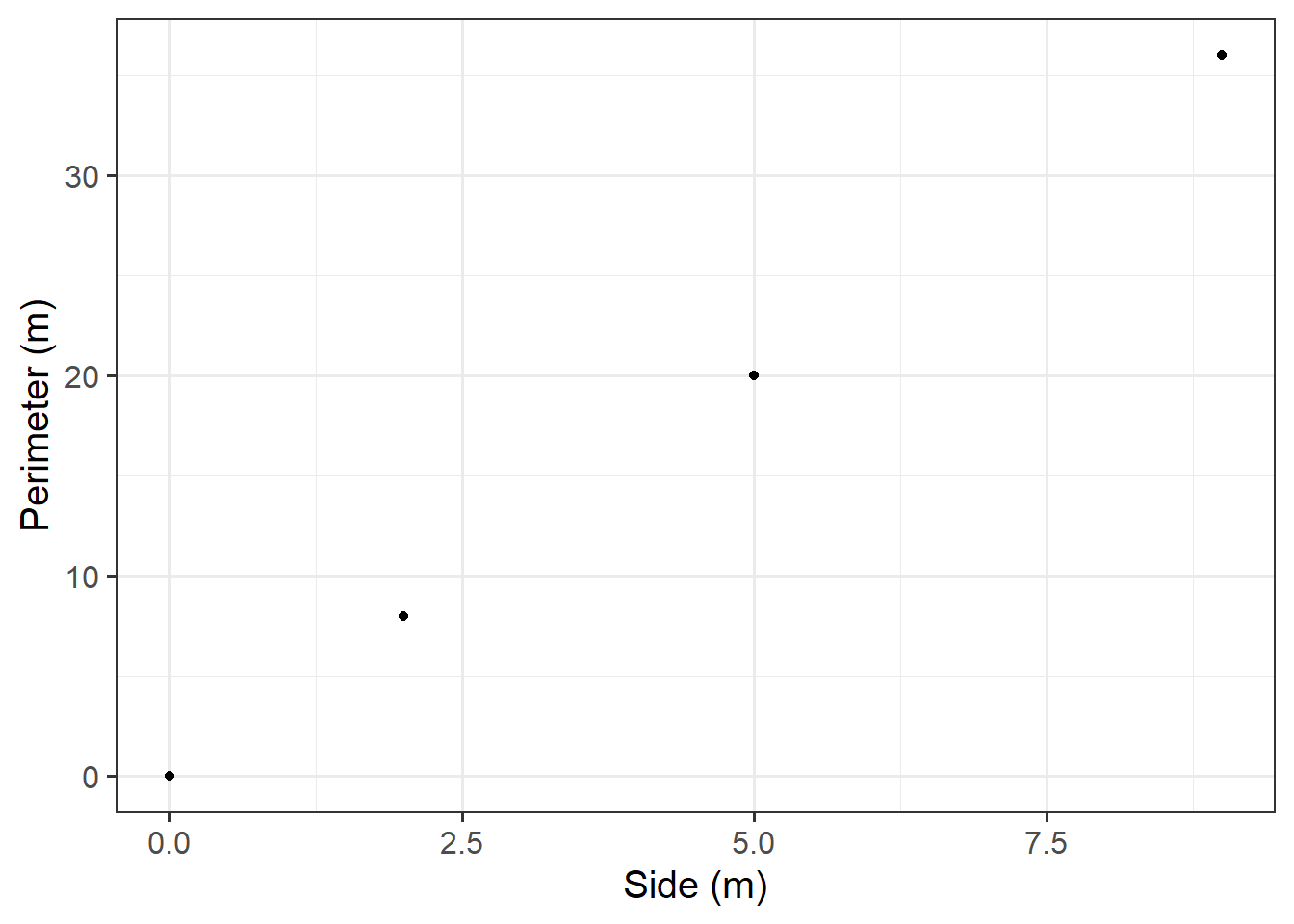
Create a data set called squares containing the perimeter of four squares having sides of length \(0, 2, 5, 9\) metres, and then plot the squares data as points

Hint

Remember that to combine multiple numbers together we use the function c().

Solution

#Create 'squares' dataset using tibble()
squares <- tibble(
  side = c(0, 2, 5, 9),
  perimeter = 4 * side
)

squares

# A tibble: 4 × 2
   side perimeter
  <dbl>     <dbl>
1     0         0
2     2         8
3     5        20
4     9        36

#Create Plot
ggplot(data = squares, aes(x = side, y = perimeter)) +
  geom_point() +
  labs(x = 'Side (m)', y = 'Perimeter (m)')

Figure 1: ?(caption)

Question 5

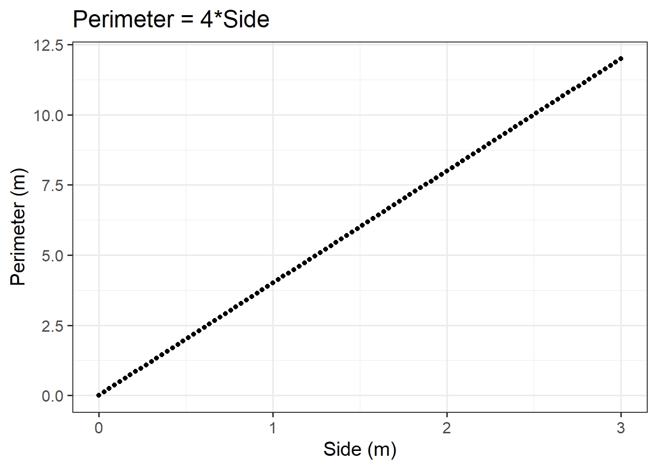
Generate one hundred data points, and use them to visualise the relationship between side and perimeter of squares. To do so, you need to complete four steps:

• Create a sequence of one hundred side lengths (x) going from 0 to 3 metres.

• Compute the corresponding perimeters (y).

• Plot the side and perimeter data as points on a graph.

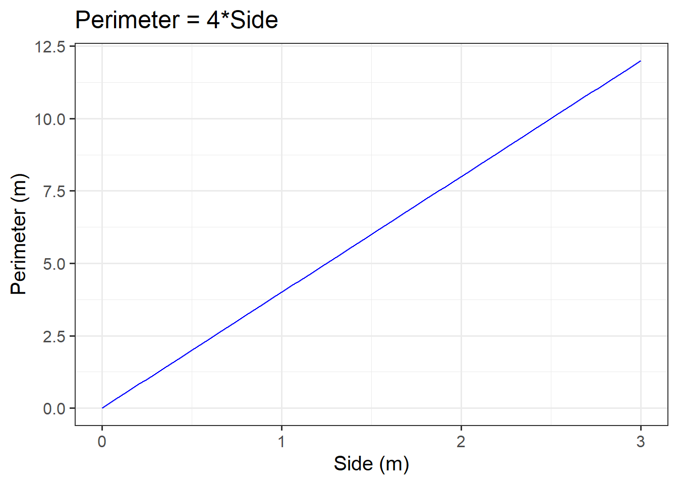
• Visualise the functional relationship between side and perimeter of squares. To do so, use the function geom_line() to connect the computed points with lines.

Hint

Remember that to create a sequence of numbers, we can use the function seq().

Solution

Let’s start by creating the side and perimeter data:

#step 1 & 2
squares_grid <- tibble(
  side = seq(0, 3, length.out = 100),
  perimeter = 4 * side
)

Plot the individual points:

# step 3
ggplot(data = squares_grid, aes(x = side, y = perimeter)) +
  geom_point() +
  labs(x = 'Side (m)', y = 'Perimeter (m)', title = 'Perimeter = 4*Side')

Visualise the functional relationship by connecting the individual points with lines:

#step 4
ggplot(data = squares_grid, aes(x = side, y = perimeter)) +
  geom_line(colour = 'blue') +
  labs(x = 'Side (m)', y = 'Perimeter (m)', title = 'Perimeter = 4*Side')

Note

The function \(y = 4 \ x\) that you plotted above is an example of a function representing a mathematical model.

We typically validate a model using experimental data. However, we all know how squares work and that two squares with the same side will have the same perimeter (more on this later).

Question 6

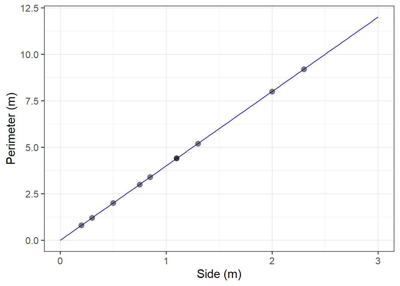
The Scottish National Gallery kindly provided us with measurements of side and perimeter (in metres) for a sample of 10 square paintings.

The data are provided below:

sng <- tibble(
  side = c(1.3, 0.75, 2, 0.5, 0.3, 1.1, 2.3, 0.85, 1.1, 0.2),
  perimeter = c(5.2, 3.0, 8.0, 2.0, 1.2, 4.4, 9.2, 3.4, 4.4, 0.8)
)

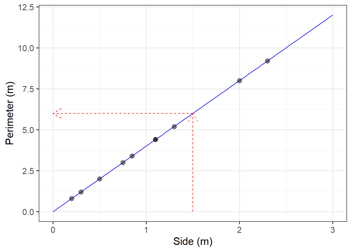
Plot the mathematical model of the relationship between side and perimeter for squares, and superimpose on top the experimental data from the Scottish National Gallery.

Solution

sng <- tibble(
  side = c(1.3, 0.75, 2, 0.5, 0.3, 1.1, 2.3, 0.85, 1.1, 0.2),
  perimeter = c(5.2, 3.0, 8.0, 2.0, 1.2, 4.4, 9.2, 3.4, 4.4, 0.8)
)

ggplot() +
  geom_line(data = squares_grid, aes(x = side, y = perimeter), colour = 'blue') +
  geom_point(data = sng, aes(x = side, y = perimeter), colour = 'black', 
             alpha = 0.5, size = 3) +
  labs(x = 'Side (m)', y = 'Perimeter (m)')

Figure 2: The exact relationship between side and perimeter of squares

The above plot shows perfect agreement between the observed data and the model.

Question 7

Use the mathematical model to predict the perimeter of a painting with a side of 1.5 metres.

Hint

Don’t forget to always include the measurement units when reporting/writing-up results!

Solution

We do not have a painting with a side of 1.5 metres within the random sample of paintings from the Scottish National Gallery. However, we can predict the perimeter of an unobserved squared painting having a 1.5 metre side using the mathematical model.

You can obtain this prediction using either a visual approach or an algebraic one.

Visual Approach

Sometimes we can directly read a predicted value from the graph of the functional relationship.

Consider the plot created in the previous question. First, we need to check where x = 1.5. Then, we draw a vertical dashed line until it meets the blue line. The y value corresponding to x = 1.5 can be read off the y-axis.

However, in this case it is not that easy to read it from the drawing…

Algebraic Approach

You can substitute the x value in the formula and calculate the corresponding y value. \[ y = 4 * x = 4 * 1.5 = 6 \]

The predicted perimeter of squared paintings having a 1.5m side is 6m.

Statistical Models

Study Overview

Research Question

How does handspan vary as a function of height?

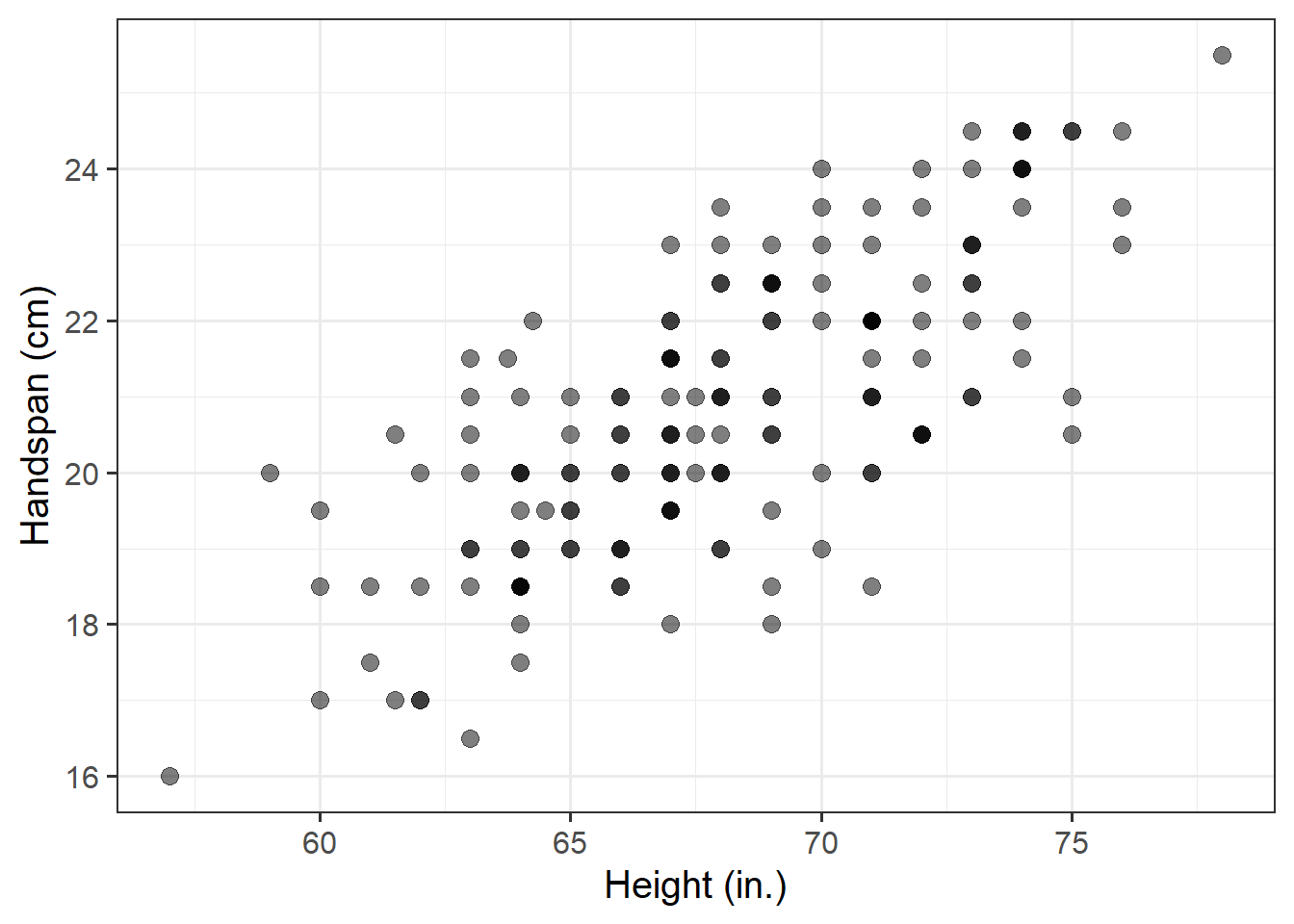
Consider now the relationship between height (in inches) and handspan (in cm). Utts and Heckard (2015) provided data for a sample of 167 students which reported their height and handspan as part of a class survey.

Using the handheight data you already loaded at the start of the lab, your task is to investigate how handspan varies as a function of height for the students in the sample.

Handheight codebook.

Description

The data set records the height and handspan reported by a random sample of 167 students as part of a class survey.

The variables are:

• height, measured in inches
• handspan, measured in centimetres

Preview

The first six rows of the data are:

height	handspan
68	21.5
71	23.5
73	22.5
64	18.0
68	23.5
59	20.0

Question 8

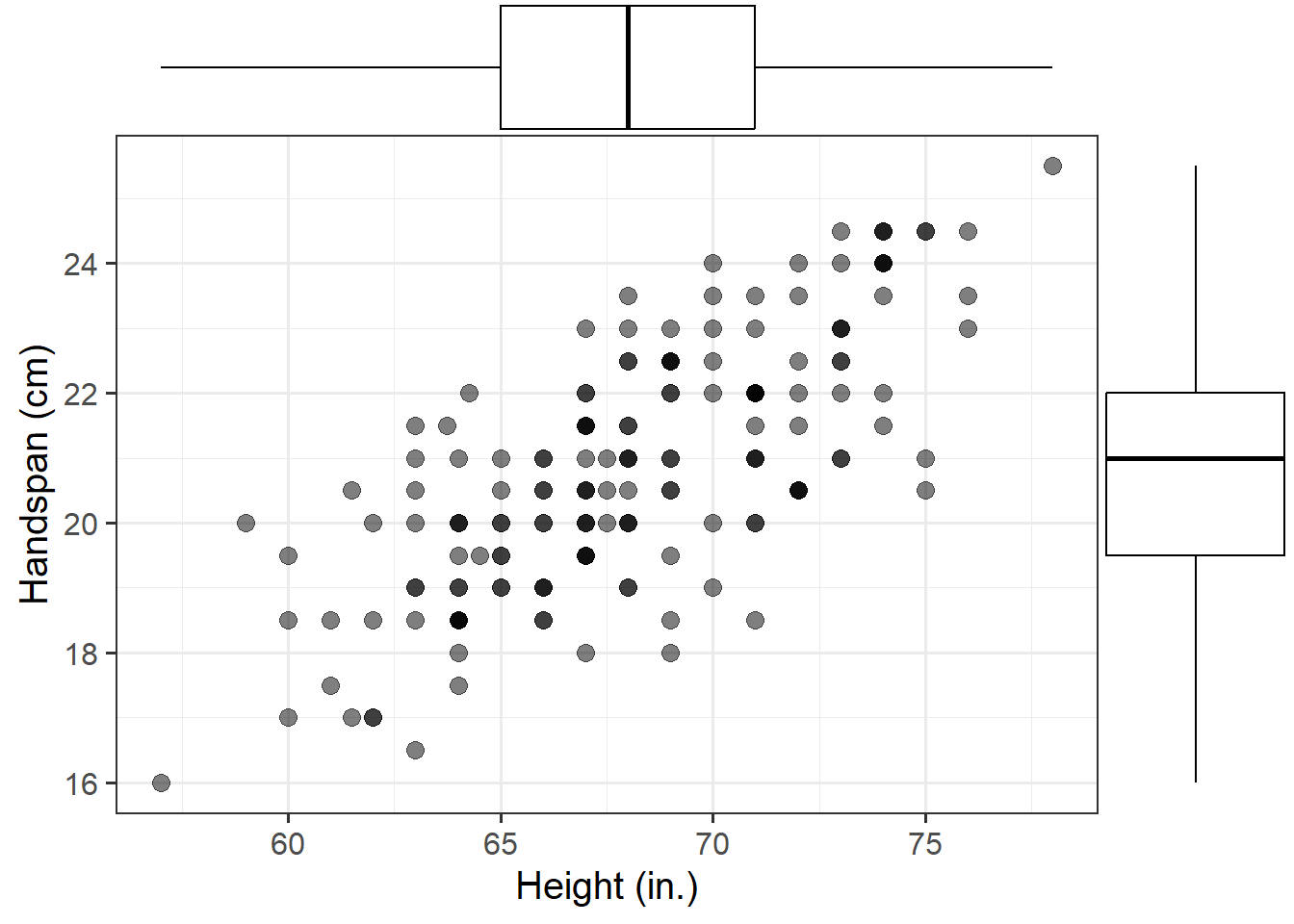
Using a scatterplot (since the variables are numeric and continuous) to visualise the relationship between the two numeric variables, comment on any main differences you notice with the relationship between side and perimeter of squares. Note if you detected outliers or points that do not fit with the pattern in the rest of the data.

Solution

plt <- ggplot(handheight, aes(x = height, y = handspan)) +
  geom_point(size = 3, alpha = 0.5) +
  labs(x = 'Height (in.)', y = 'Handspan (cm)')

plt

Figure 3: Simple Scatterplot

We can also add marginal boxplots for each variable using the package ggExtra.

ggMarginal(plt, type = 'boxplot')

Warning: Continuous x aesthetic
ℹ did you forget `aes(group = ...)`?
Continuous x aesthetic
ℹ did you forget `aes(group = ...)`?

Figure 4: The statistical relationship between height and handspan

Outliers are extreme observations that are not possible values of a variable or that do not seem to fit with the rest of the data. This could either be:

• marginally along one axis: points that have an unusual (too high or too low) x-coordinate or y-coordinate;
• jointly: observations that do not fit with the rest of the point cloud.

The boxplots in Figure 4 do not highlight any outliers in the marginal distributions of height and handspan. Furthermore, from the scatterplot we do not notice any extreme observations or points that do not fit with the rest of the point cloud.

We notice a moderate, positive linear relationship between height and handspan.

Recall Figure 2, displaying the relationship between side and perimeters of squares. In the plot we notice two points on top of each other, reflecting the fact that two squares having the same side will always have the same perimeter. In fact, the data from the Scottish National Gallery include two squared paintings with a side of 1.1m, both having a measured perimeter of 4.4m.

Figure 4, instead, displays the relationship between height and handspan of a sample of students. The first thing that grabs our attention is the fact that students having the same height do not necessarily have the same handspan. Rather, we clearly see a variety of handspan values for students all having a height of, for example, 70in. To be more precise, the seven students who are 70 in. tall all have differing handspans.

Question 9

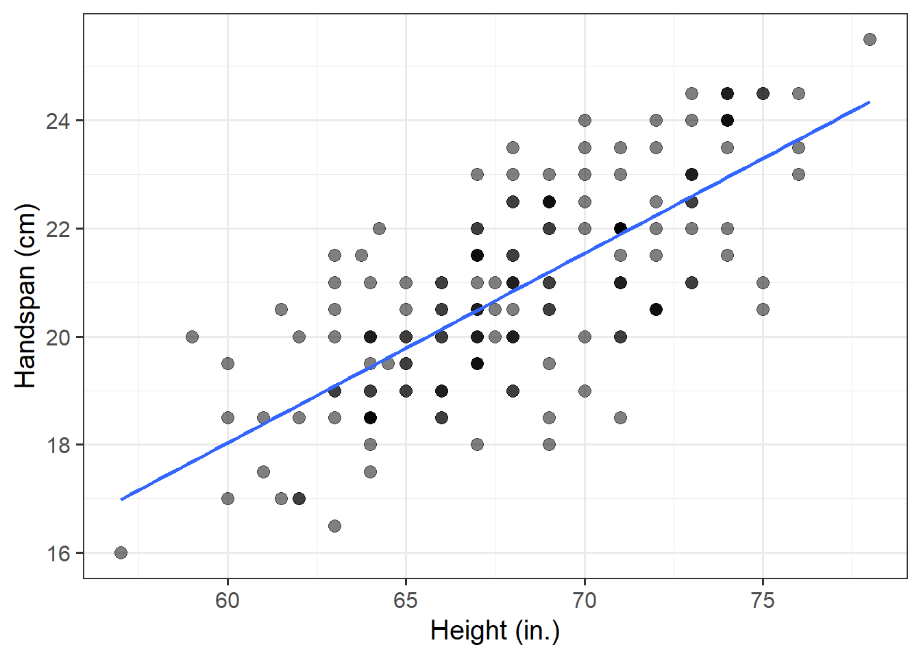
Using the following command, superimpose on top of the scatterplot a best-fit line describing how handspan varies as a function of height. For the moment, the argument se = FALSE tells R to not display uncertainty bands.

geom_smooth(method = lm, se = FALSE)

Comment on any differences between the lines representing the linear relationship between (a) the side and perimeter of square and (b) height and handspan.

Solution

ggplot(handheight, aes(x = height, y = handspan)) +
  geom_point(size = 3, alpha = 0.5) +
  geom_smooth(method = lm, se = FALSE) +
  labs(x = 'Height (in.)', y = 'Handspan (cm)')

Figure 5: The best-fit line

The line representing the relationship between side and perimeter of squares is able to predict the actual perimeter value from the measurement of the side of a square. This is possible because the relationship between side and perimeter is an exact one.

That is, any squares having the same side will have the same perimeter, and there will be no variation in those values.

The line that best fits the relationship between height and handspan (see Figure 5), instead, is only able to predict the average handspan for a given value of height.

This is because there will be a distribution of handspans at each value of height. The line will fit the trend/pattern in the values, but there will be individual-to-individual variability that we must accept around that average pattern.

Question 10

The line of best-fit is given by:¹

\[ \widehat{Handspan} = -3 + 0.35 \ Height \]

Calculate the predicted handspan of a student who is (a) 73in tall, and (b) 5in tall.

Solution

• The predicted average handspan for students who are 73in tall is:
  \(-3 + 0.35 * 73 = 22.55\)cm.
  
  
• The predicted average handspan for students who are 5in tall is:
  \(-3 + 0.35 * 5 = -1.25\)cm.

But wait, handspan can not be negative… This does not make any sense! That’s right, we went too far off the range of the available data on heights, which were between 57in and 78in. We extrapolated. This is very dangerous…

Source: Randall Munroe, xkcd.com

References

Utts, Jessica M, and Robert F Heckard. 2015. Mind on Statistics. Cengage Learning.

Footnotes

1. Yes, the error term is gone. This is because the line of best-fit gives you the prediction of the average handspan for a given height, and not the individual handspan of a person, which will almost surely be different from the prediction of the line.