Categorical Predictors & Block 1 Recap

Learning Objectives

At the end of this lab, you will:

1. Understand the meaning of (and how to interpret) a multiple regression model with a binary predictor
2. Understand how to specify a new baseline/reference level for categorical variables

What You Need

1. Be up to date with lectures
2. Have completed Labs 1 - 4

Required R Packages

Remember to load all packages within a code chunk at the start of your RMarkdown file using library(). If you do not have a package and need to install, do so within the console using install.packages(" "). For further guidance on installing/updating packages, see Section C here.

For this lab, you will need to load the following package(s):

• tidyverse
• patchwork
• sjPlot

Lab Data

You can download the data required for this lab here or read it in via this link https://uoepsy.github.io/data/wellbeing.csv.

Note: this is the same data as Lab 3 & 4.

Section A: Numeric + Categorical

Study Overview

Research Question

Is there an assocation between well-being and time spent outdoors after taking into account the assocation between well-being and having a routine?

Wellbeing data codebook.

Description

Researchers interviewed 32 participants, selected at random from the population of residents of Edinburgh & Lothians. They used the Warwick-Edinburgh Mental Wellbeing Scale (WEMWBS), a self-report measure of mental health and well-being. The scale is scored by summing responses to each item, with items answered on a 1 to 5 Likert scale. The minimum scale score is 14 and the maximum is 70.

The researchers also asked participants to estimate the average number of hours they spend outdoors each week, the average number of social interactions they have each week (whether on-line or in-person), and whether they believe that they stick to a routine throughout the week (Yes/No).

The data in wellbeing.csv contain five attributes collected from a random sample of \(n=32\) hypothetical residents over Edinburgh & Lothians, and include:

• wellbeing: Warwick-Edinburgh Mental Wellbeing Scale (WEMWBS), a self-report measure of mental health and well-being. The scale is scored by summing responses to each item, with items answered on a 1 to 5 Likert scale. The minimum scale score is 14 and the maximum is 70.
  
• outdoor_time: Self report estimated number of hours per week spent outdoors
  
• social_int: Self report estimated number of social interactions per week (both online and in-person)
• routine: Binary Yes/No response to the question “Do you follow a daily routine throughout the week?”
• location: Location of primary residence (City, Suburb, Rural)

Preview

The first six rows of the data are:

wellbeing	outdoor_time	social_int	location	routine
30	7	8	Suburb	Routine
21	9	8	City	No Routine
38	14	10	Suburb	Routine
27	16	10	City	No Routine
20	1	10	Rural	No Routine
37	11	12	Suburb	No Routine

Setup

Setup

1. Create a new RMarkdown file
2. Load the required package(s)
3. Read the wellbeing dataset into R, assigning it to an object named mwdata
4. Check coding of variables (e.g., make sure that catgorical variables are coded as factors)

Hint

You will need to use the as_factor() function here. Note that this function creates levels from the order in which they appear in your dataset (e.g., routine is in the first row of our mwdata, so would be assigned as the reference group).

Solution

#Loading the required package(s)
library(tidyverse)
library(patchwork)
library(sjPlot)

# Reading in data and storing to an object named 'mwdata'
mwdata <- read_csv("https://uoepsy.github.io/data/wellbeing.csv")

#check coding of routine variable - should be a factor - check by running `is.factor()`
is.factor(mwdata$routine) #result = false, so need to make routine a factor

[1] FALSE

#designate routine as factor and check using above code if change has been applied by re-running line (should now be TRUE)
mwdata$routine <- as_factor(mwdata$routine)

Question 1

Produce visualisations of:

1. the distribution of the routine variable
2. the association between routine and wellbeing.

Provide interpretation of these figures.

Note

We cannot visualise the distribution of routine as a density curve or boxplot, because it is a categorical variable (observations can only take one of a set of discrete response values). Revise the DAPR1 materials for a recap of data types.

Hint

Consider using geom_bar() and/or geom_boxplot(). The DAPR1 categorical data lab might provide a useful starting point if needed.

Solution

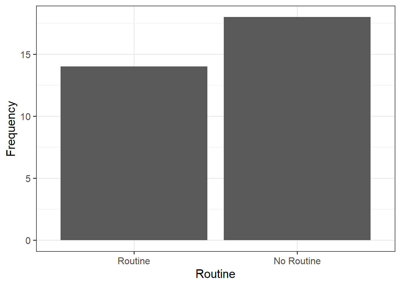
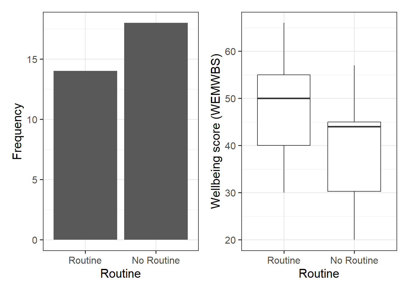
geom_bar() will count the number of observations falling into each unique level of the routine variable:

p1 <- ggplot(data = mwdata, aes(x = routine)) +
  geom_bar()+
  labs(x = "Routine", y = "Frequency")
p1

Figure 1: Marginal distribution plots of Routine (y/n)

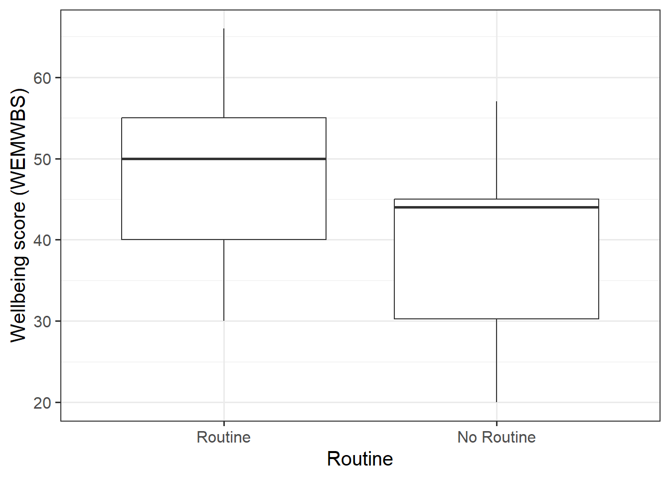
We might plot the association between routine and wellbeing as two boxplots:

p2 <- ggplot(data = mwdata, aes(x = routine, y = wellbeing)) +
  geom_boxplot()+
  labs(x = "Routine", y = "Wellbeing score (WEMWBS)")
p2

Figure 2: Relationship between wellbeing and presence of routine

#place plots adjacent to one another
p1 | p2

From Figure 1, we can see that there are more individuals that do not have a routine than those who do.

From Figure 2, we can see that individuals with a routine tend to have higher wellbeing scores than those who do not.

Question 2

1. Formally state:

• your chosen significance level
• the null and alternative hypotheses

2. Fit the multiple regression model below using lm(), and assign it to an object named mdl2.

\[ Wellbeing = \beta_0 + \beta_1 \cdot Routine_{No Routine} + \beta_2 \cdot OutdoorTime + \epsilon \]

Examine the summary() output of the model.

\(\hat \beta_0\) (the intercept) is the estimated average wellbeing score associated with zero hours of weekly outdoor time and zero in the routine variable. What group is the intercept the estimated wellbeing score for when they have zero hours of outdoor time? Why (think about what zero in the routine variable means)?

Solution

Effects will be considered statistically significant at \(\alpha=.05\)

\(H_0: \beta_2 = 0\)

There is no association between well-being and time spent outdoors after taking into account the relationship between well-being and routine

\(H_1: \beta_2 \neq 0\)

There is an association between well-being and time spent outdoors after taking into account the relationship between well-being and routine

mdl2 <- lm(wellbeing ~  routine + outdoor_time, data = mwdata)
summary(mdl2)

Call:
lm(formula = wellbeing ~ routine + outdoor_time, data = mwdata)

Residuals:
     Min       1Q   Median       3Q      Max 
-16.3597  -5.7983   0.1047   7.2899  12.5957 

Coefficients:
                  Estimate Std. Error t value Pr(>|t|)    
(Intercept)        33.5472     4.4263   7.579 2.35e-08 ***
routineNo Routine  -7.2947     3.2507  -2.244 0.032633 *  
outdoor_time        0.9152     0.2358   3.881 0.000552 ***
---
Signif. codes:  0 '***' 0.001 '**' 0.01 '*' 0.05 '.' 0.1 ' ' 1

Residual standard error: 9.06 on 29 degrees of freedom
Multiple R-squared:  0.4361,    Adjusted R-squared:  0.3972 
F-statistic: 11.21 on 2 and 29 DF,  p-value: 0.0002467

As you can see in the output of the model, we have a coefficient called routineNo Routine. This is the parameter estimate for a dummy variable which has been inputted into the model. The lm() function will automatically name the dummy variables (and therefore the coefficients) according to what level is identified by the 1. It names them <variable><Level>, so we can tell that routineNo Routine is 1 for “No Routine” and 0 for “Routine”.

The intercept is therefore the estimated wellbeing score for those with a Routine and zero hours of outdoor time.

Question 3

The researchers have decided that they would prefer ‘no routine’ to be considered the reference level for the “routine” variable instead of ‘routine’. Apply this change to the variable and re-run your model.

Hint

You will need to use the relevel() function here.

Solution

Now we are fitting the below model:

\[ Wellbeing = \beta_0 + \beta_1 \cdot Routine_{Routine} + \beta_2 \cdot OutdoorTime + \epsilon \] So we will need to change our reference group before re-running out model:

#re-order so that no routine is reference level
mwdata$routine <- relevel(mwdata$routine, 'No Routine')

#re-run model and check summary
mdl2_reorder <- lm(wellbeing ~  routine + outdoor_time, data = mwdata)
summary(mdl2_reorder)

Call:
lm(formula = wellbeing ~ routine + outdoor_time, data = mwdata)

Residuals:
     Min       1Q   Median       3Q      Max 
-16.3597  -5.7983   0.1047   7.2899  12.5957 

Coefficients:
               Estimate Std. Error t value Pr(>|t|)    
(Intercept)     26.2525     3.9536   6.640  2.8e-07 ***
routineRoutine   7.2947     3.2507   2.244 0.032633 *  
outdoor_time     0.9152     0.2358   3.881 0.000552 ***
---
Signif. codes:  0 '***' 0.001 '**' 0.01 '*' 0.05 '.' 0.1 ' ' 1

Residual standard error: 9.06 on 29 degrees of freedom
Multiple R-squared:  0.4361,    Adjusted R-squared:  0.3972 
F-statistic: 11.21 on 2 and 29 DF,  p-value: 0.0002467

You should now see that our routine variable is now showing routineRoutine instead of routineNo Routine. This means that 1 is now for “Routine” and 0 for “No Routine”.

Question 4

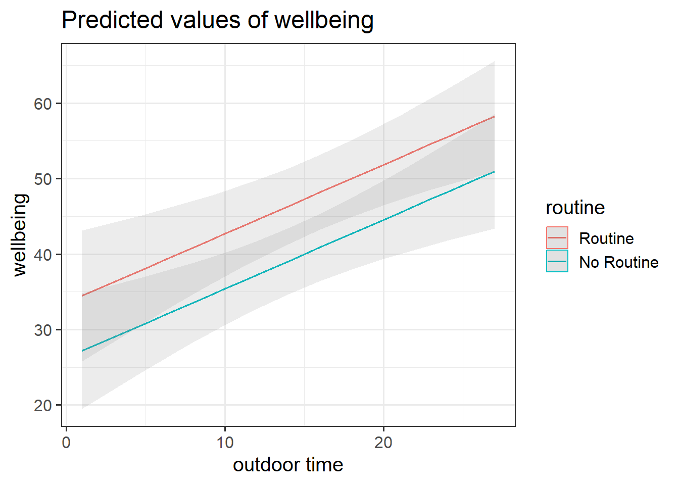
We can visualise the model below as two lines.

\(\widehat{Wellbeing} = \hat \beta_0 + \hat \beta_1 \cdot Routine_{Routine} + \hat \beta_2 \cdot OutdoorTime\)

Each line represents the model predicted values for wellbeing scores across the range of weekly outdoor time, with one line for those who report having “Routine” and one for those with “No Routine”.

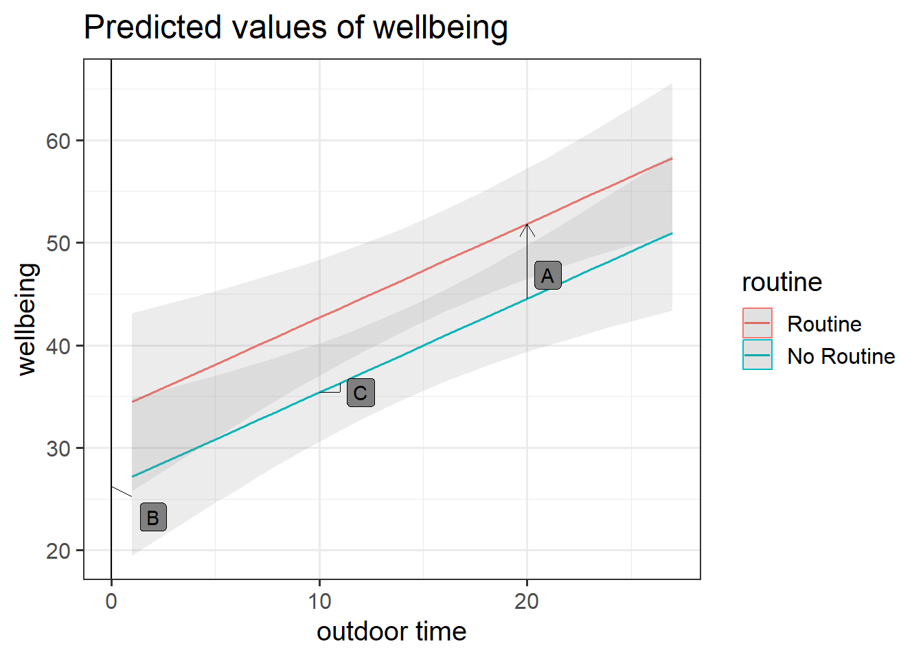
Get a pen and paper, and sketch out the plot shown in Figure 3.

Figure 3: Multiple regression model: Wellbeing ~ Routine + Outdoor Time

Annotate your plot with labels for each of parameter estimates from your model:

Parameter Estimate	Model Coefficient	Estimate
\(\hat \beta_0\)	(Intercept)	26.25
\(\hat \beta_1\)	routineRoutine	7.29
\(\hat \beta_2\)	outdoor_time	0.92

Hint

Below you can see where to add the labels, but we have not said which is which.

• A is the vertical distance between the red and blue lines (the lines are parallel, so this distance is the same wherever you cut it on the x-axis).
  
• B is the point at which the blue line cuts the y-axis.
  
• C is the vertical increase (increase on the y-axis) for the blue line associated with a 1 unit increase on the x-axis (the lines are parallel, so this is the same for the red line).

Solution

• A = \(\hat \beta_2\) = routineRoutine coefficient = 7.29
• B = \(\hat \beta_0\) = (Intercept) coefficient = 26.25
• C = \(\hat \beta_1\) = outdoor_time coefficient = 0.92

Question 5

Interpret your results in the context of the research question and report your model in full.

Provide key model results in a formatted table.

Solution

#create table for results
tab_model(mdl2_reorder,
          dv.labels = "Wellbeing (WEMWBS Scores)",
          pred.labels = c("routineRoutine" = "Has Routine",
                          "outdoor_time" = "Outdoor Time (hours per week)"),
          title = "Regression Table for Wellbeing Model")

Table 1: Regression Table for Wellbeing Model

	Wellbeing (WEMWBS Scores)
Predictors	Estimates	CI	p
(Intercept)	26.25	18.17 – 34.34	<0.001
Has Routine	7.29	0.65 – 13.94	0.033
Outdoor Time (hours per week)	0.92	0.43 – 1.40	0.001
Observations	32
R2 / R2 adjusted	0.436 / 0.397

And now lets write our results up:

Full regression results including 95% Confidence Intervals are shown in Table 1. The \(F\)-test for model utility was significant \((F(2,29) = 11.21, p<.001)\), and the model explained approximately 39.72% of the variability in wellbeing scores.

After controlling for routine, there was a significant association between wellbeing scores and outdoor time \((\beta = 0.92, SE = 0.24, p < .001)\). This suggested that for every additional hour of outdoor time, wellbeing scores, on average, were higher by 0.92 points (\(CI_{95}[0.43 - 1.40]\)). Therefore, we have evidence to reject the null hypothesis (that there was no association between well-being and time spent outdoors after taking into account the relationship between well-being and routine).

Section B: Weeks 1 - 4 Recap

In the second part of the lab, there is no new content - the purpose of the recap section is for you to revisit and revise the concepts you have learned over the last 4 weeks.

Before you expand each of the boxes below, think about how comfortable you feel with each concept.

Types of Models: Deterministic vs Statistical

Deterministic (Example: Perimeter & Side)

The mathematical model

\[ Perimeter = 4 * Side \]

or, equivalently, \[ y = 4 * x \]

represents the relationship between side and perimeter of squares. This is an example of a deterministic model as it is a model of an exact relationship - there can be no deviation.

Statistical (Example: Height & Handspan)

The relationship between height and handspan shows deviations from the ‘average pattern’. Hence, we need to create a model that allows for deviations from the linear relationship - we need a statistical model.

A statistical model includes both a deterministic function and a random error term: \[ Handspan = \beta_0 + \beta_1 * Height + \epsilon \] or, in short, \[ y = \underbrace{\beta_0 + \beta_1 * x}_{\text{function of }x} + \underbrace{\epsilon}_{\text{random error}} \]

The deterministic function need not be linear if the scatterplot displays signs of nonlinearity.

In the equation above, the terms \(\beta_0\) and \(\beta_1\) are numbers specifying where the line going through the data meets the y-axis and its slope (direction and gradient of line).

Note

See Week 1 lab and both lecture 1 and lecture 2 for further details and to revise these concepts further.

Null & Alternative Hypotheses

Recall that statistical hypotheses are testable mathematical statements.

We need to define a null (\(H_0\)) and alternative (\(H_1\)) hypothesis.

Points to note:

• We can only ever test the null (\(H_0\)), so all statements must be made in reference to this
• We can only ever reject or fail to reject the null (we can never accept a hypothesis)

Simple Linear Regression

Formula:

\[ y_i = \beta_0 + \beta_1 x_i + \epsilon_i \] In R:

There are basically two pieces of information that we need to pass to the lm() function:

1. The formula: The regression formula should be specified in the form y ~ x where \(y\) is the dependent variable (DV) and \(x\) the independent variable (IV).
2. The data: Specify which dataframe contains the variables specified in the formula.

• run simple linear regression via lm() function

model_name <- lm(DV ~ IV, data = data_name)

OR

model_name <- lm(data_name$DV ~ data_name$IV)

Note

See Week 2 lab and lectures for further details, examples, and to revise these concepts further.

Multiple Linear Regression

Formula:

\[ y_i = \beta_0 + \beta_1 x_1 + \beta_2 x_2 + \epsilon_i \] In R:

Multiple and simple linear regression follow the same structure within the lm() function. You simply add (using the + sign) more independent variables.

• run multiple linear regression (example includes three independent variables) via lm() function

model_name <- lm(DV ~ IV1 + IV2 + IV3, data = data_name)

OR

model_name <- lm(data_name$DV ~ data_name$IV1 + data_name$IV2 + data_name$IV3

Interpretation of Multiple Regression Coefficients

You’ll hear a lot of different ways that people explain multiple regression coefficients.

For the model \(y = \beta_0 + \beta_1 x_1 + \beta_2 x_2 + \epsilon\), the estimate \(\hat \beta_1\) will often be reported as:

the increase in \(y\) for a one unit increase in \(x_1\) when…

• holding the effect of \(x_2\) constant.
• controlling for differences in \(x_2\).
• partialling out the effects of \(x_2\).
• holding \(x_2\) equal.
• accounting for effects of \(x_2\).

Note

See Week 3 lab and lectures for further details, examples, and to revise these concepts further.

Partitioning Variation: Sum of Squares

Sum of Squares

The sum of squares measures the deviation or variation of data points away from the mean (i.e., how spread out are the numbers in a given dataset). We are trying to find the equation/function that best fits our data by varying the least from our data points.

Total Sum of Squares

Formula:

\[SS_{Total} = \sum_{i=1}^{n}(y_i - \bar{y})^2\]

In words:

Squared distance of each data point from the mean of \(y\).

Description:

How much variation there is in the DV.

Residual Sum of Squares

Formula:

\[SS_{Residual} = \sum_{i=1}^{n}(y_i - \hat{y}_i)^2\]

In words:

Squared distance of each point from the predicted value.

Description:

How much of the variation in the DV the model did not explain - a measure that captures the unexplained variation in your regression model. Lower residual sum of squares suggests that your model fits the data well, and higher suggests that the model poorly explains the data (in other words, the lower the value, the better the regression model). If the value was zero here, it would suggest the model fits perfectly with no error.

Model Sum of Squares

Formula:

\[SS_{Model} = \sum_{i=1}^{n}(\hat{y}_i - \bar{y})^2\]

Can also be derived from:

\[SS_{Model} = SS_{Total} - SS_{Residual}\] In words:

The deviance of the predicted scores from the mean of \(y\).

Description:

How much of the variation in the DV your model explained - like a measure that captures how well the regression line fits your data.

Note

See Week 3 lab and lectures, as well as Week 4 lab and lectures for further details, examples, and to revise these concepts further.

F-test & F-ratio

Formula:

\[ F_{df_{model},df_{residual}} = \frac{MS_{Model}}{MS_{Residual}} = \frac{SS_{Model}/df_{Model}}{SS_{Residual}/df_{Residual}} \\ \quad \\ \begin{align} & \text{Where:} \\ & df_{model} = k \\ & df_{residual} = n-k-1 \\ & n = \text{sample size} \\ & k = \text{number of explanatory variables} \\ \end{align} \] Description:

To test the significance of an overall model, we can conduct an \(F\)-test. The \(F\)-test compares your model to a model containing zero predictor variables (i.e., the intercept only model), and tests whether your added predictor variables significantly improved the model.

The \(F\)-test involves testing the statistical significance of the \(F\)-ratio. Q: What does the \(F\)-ratio test? A: The null hypothesis that all regression slopes in a model are zero (i.e., explain no variance in your outcome/DV).

Points to note:

• The larger your \(F\)-ratio, the better your model
• The \(F\)-ratio will be close to 1 when the null is true (i.e., that all slopes are zero)

Interpretation:

If your model predictors do explain some variance, the \(F\)-ratio will be significant, and you would reject the null, as this would suggest that your predictor variables included in your model improved the model fit (in comparison to the intercept only model).

Note

See Week 4 lab and lectures for further details, examples, and to revise these concepts further.

R-squared and Adjusted R-squared

\(R^2\) represents the proportion of variance in \(Y\) that is explained by the model.

The \(R\)-squared coefficient is defined as: \[ R^2 = \frac{SS_{Model}}{SS_{Total}} = 1 - \frac{SS_{Residual}}{SS_{Total}} \]

The Adjusted \(R\)-squared coefficient is defined as: \[ \hat R^2 = 1 - \frac{(1 - R^2)(n-1)}{n-k-1} \quad \\ \begin{align} & \text{Where:} \\ & n = \text{sample size} \\ & k = \text{number of explanatory variables} \\ \end{align} \] We can see the Multiple and Adjusted \(R\)-squared in the summary() output of a model.

Points to note:

• Adjusted-\(R^2\) adjusts for the number of terms in a model, and should be used when there are 2 or more predictors in the model
• Adjusted-\(R^2\) should always be less than or equal to \(R^2\)

Note

See Week 4 lab and lectures for further details, examples, and to revise these concepts further.

Standardisation

\(z\)-score Formula:

\[ z_x = \frac{x - \bar{x}}{s_x}, \qquad z_y = \frac{y - \bar{y}}{s_y} \]

Recall that a standardized variable has mean of 0 and standard deviation of 1.

In R:

#create z-scored variables
dataframe <- dataframe %>%
  mutate(
   z_variable = (variable - mean(variable)) / sd(variable)
    )

OR

#use scale function
model <- lm(scale(DV) ~ scale(IV), data = dataset)

Note

See Week 4 lab and lectures for further details, examples, and to revise these concepts further.

Binary Variables

Binary predictors in linear regression

We can include categorical predictors in a linear regression, but the interpretation of the coefficients is very specific. Whereas we talked about coefficients being interpreted as “the change in \(y\) associated with a 1-unit increase in \(x\)”, for categorical explanatory variables, coefficients can be considered to examine differences in group means. However, they are actually doing exactly the same thing - the model is simply translating the levels (like “Yes”/“No”) in to 0s and 1s!

Our coefficients are just the same as before. The intercept is where our predictor equals zero, and the slope is the change in our outcome variable associated with a 1-unit change in our predictor.

However, “zero” for this predictor variable now corresponds to a whole level. This is known as the “reference level”. Accordingly, the 1-unit change in our predictor (the move from “zero” to “one”) corresponds to the difference between the two levels.

Note

See Week 5 lab and lectures for further details, examples, and to revise these concepts further.

Categorical Predictors with k levels

We saw that a binary categorical variable gets inputted into our model as a variable of 0s and 1s (these typically get called “dummy variables”).

Dummy variables are numeric variables that represent categorical data.

When we have a categorical explanatory variable with more than 2 levels, our model gets a bit more - it needs not just one, but a number of dummy variables. For a categorical variable with \(k\) levels, we can express it in \(k-1\) dummy variables.

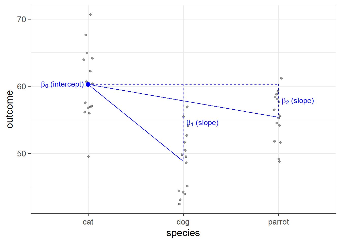
For example, the “species” column below has three levels, and can be expressed by the two variables “species_dog” and “species_parrot”:

  species species_dog species_parrot
1     cat           0              0
2     cat           0              0
3     dog           1              0
4  parrot           0              1
5     dog           1              0
6     cat           0              0
7     ...         ...            ...

• The “cat” level is expressed whenever both the “species_dog” and “species_parrot” variables are 0.
• The “dog” level is expressed whenever the “species_dog” variable is 1 and the “species_parrot” variable is 0.
• The “parrot” level is expressed whenever the “species_dog” variable is 0 and the “species_parrot” variable is 1.

R will do all of this re-expression for us. If we include in our model a categorical explanatory variable with 4 different levels, the model will estimate 3 parameters - one for each dummy variable. We can interpret the parameter estimates (the coefficients we obtain using coefficients(),coef() or summary()) as the estimated increase in the outcome variable associated with an increase of one in each dummy variable (holding all other variables equal).

	Estimate	Std. Error	t value	Pr(>|t|)
(Intercept)	60.28	1.209	49.86	5.273e-39
speciesdog	-11.47	1.71	-6.708	3.806e-08
speciesparrot	-4.916	1.71	-2.875	0.006319

Note that in the above example, an increase in 1 of “species_dog” is the difference between a “cat” and a “dog”. An increase in one of “species_parrot” is the difference between a “cat” and a “parrot”. We think of the “cat” category in this example as the reference level - it is the category against which other categories are compared against.

Note

See Week 5 lectures for further details, examples, and to revise these concepts further.

Steps Involved in Modelling

You can think of the sequence of steps involved in statistical modeling as:
\[ \text{Choose} \rightarrow \text{Fit} \rightarrow \text{Assess} \rightarrow \text{Use} \]

A general rule

Do not use (draw inferences or predictions from) a model before you have assessed whether the model satisfies the underlying assumptions

Throughout this block, we have completed the first three steps (Choose, Fit, and Use) in that we have:

1. Explored/visualised our data and specified our model
2. Fitted the model in R
   
3. Interpreted our parameter estimates

Please note that when conducting real analyses, it would be inappropriate to complete these steps without also assessing whether a regression model meets the assumptions. You will learn how to do this in Block 2 of Semester 1 for linear regression models.