Assumptions and Diagnostics

Learning Objectives

At the end of this lab, you will:

1. Be able to state the assumptions underlying a linear model.
2. Specify the assumptions underlying a linear model with multiple predictors.
3. Assess if a fitted model satisfies the assumptions of your model.
4. Assess the effect of influential cases on linear model coefficients and overall model evaluations.

What You Need

1. Be up to date with lectures
2. Have completed previous lab exercises from Week 7, Week 8, and Week 9

Required R Packages

Remember to load all packages within a code chunk at the start of your RMarkdown file using library(). If you do not have a package and need to install, do so within the console using install.packages(" "). For further guidance on installing/updating packages, see Section C here.

For this lab, you will need to load the following package(s):

• tidyverse
• car
• see
• performance

Lab Data

You can download the data required for this lab here and here or read both datsets in via these links https://uoepsy.github.io/data/riverview.csv and https://uoepsy.github.io/data/wellbeing.csv.

Lab Overview

In the previous labs, we have fitted a number of regression models, including some with multiple predictors. In each case, we first specified the model, then visually explored the marginal distributions and relationships of variables which would be used in the analysis. Finally, we fit the model, and began to examine the fit by studying what the various parameter estimates represented, and the spread of the residuals.

But before we draw inferences using our model estimates or use our model to make predictions, we need to be satisfied that our model meets a specific set of assumptions. If these assumptions are not satisfied, the results will not hold.

In this lab, we will check the assumptions of two models that we have previously fitted - one simple linear model, and one with multiple predictors. Specifically, we will check the assumptions from the simple linear regression model we fitted using the ‘riverview’ dataset in Week 2, and the assumptions of the multiple linear regression model we fitted using the ‘wellbeing’ dataset in Week 3.

Setup

Setup

1. Create a new RMarkdown file
2. Load the required package(s)
3. Read the riverview and wellbeing datasets into R, assigning them to objects named rvdata and wbdata respectively
4. Fit the following models:

\[ Model 1: Income = \beta_0 + \beta_1 \ Education \]

\[ Model 2: Wellbeing = \beta_0 + \beta_1 Social Interactions + \beta_2 Outdoor Time \\ \]

Solution

#Loading the required package(s)
library(tidyverse)
library(car)
library(see)
library(performance)

#Reading in data and storing in object named 'rvdata' and 'wbdata'
rvdata <- read_csv("https://uoepsy.github.io/data/riverview.csv")
wbdata <-  read_csv("https://uoepsy.github.io/data/wellbeing.csv")

#fit models
## riverview model
rv_mdl1 <- lm(income ~ education, data = rvdata) 

## wellbeing model
wb_mdl1 <- lm(wellbeing ~ outdoor_time + social_int, data = wbdata) 

Exercises

Assumptions

Assumptions

You can remember the four assumptions by memorising the acronym LINE:

• Linearity: The relationship between \(y\) and \(x\) is linear.
• Independence of errors: The error terms should be independent from one another.
• Normality: The errors \(\epsilon\) are normally distributed in the population.
• Equal variances (“Homoscedasticity”): The variability of the errors \(\epsilon\) is constant across \(x\).

Question 1

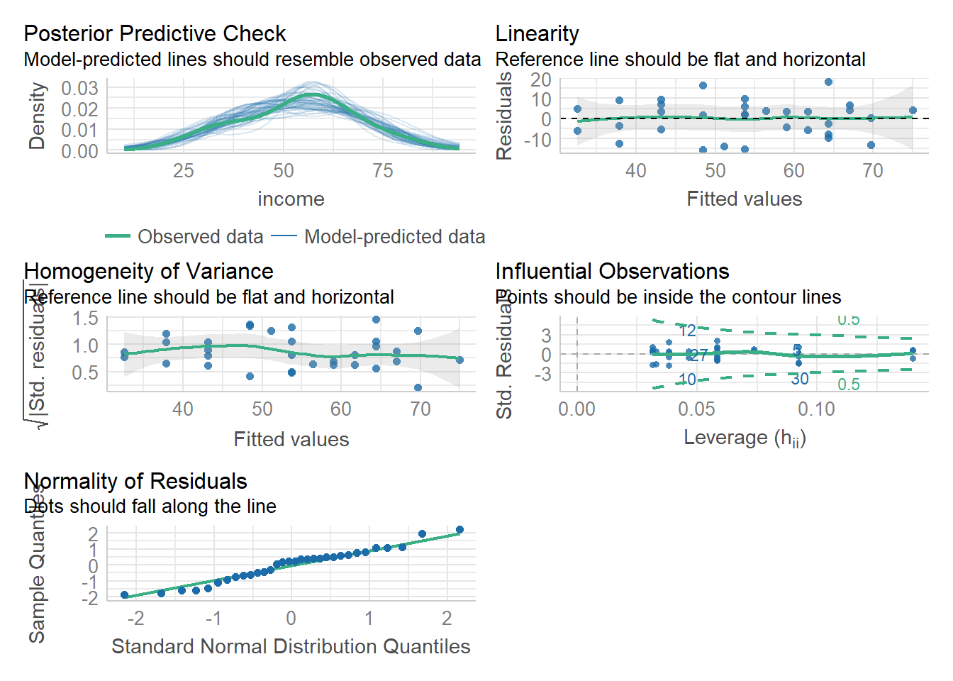
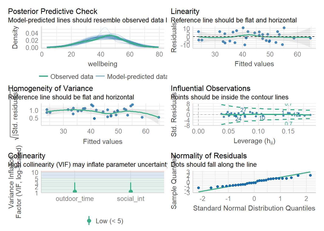
Let’s start by using check_model() for both rv_mdl1 and wb_mdl1 models - we can refer to these plots as a guide as we work through the assumptions questions of the lab.

These plots cannot be used in your reports - they are to be used as a guide only.

Solution

rv_mdl1 model

check_model(rv_mdl1)

wb_mdl1 model

check_model(wb_mdl1)

Variable `Component` is not in your data frame :/

The check_model() function is a useful way to check the assumptions of models, as it also returns some useful notes to aid your interpretation. From the above, it doesn’t appear that any of the assumptions for either have been violated, but we need to check each assumption individually with plots that are more suitable for a statistics report.

Question 2

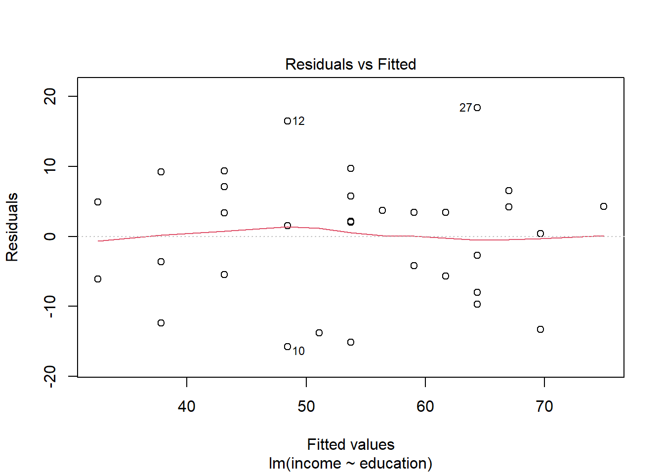
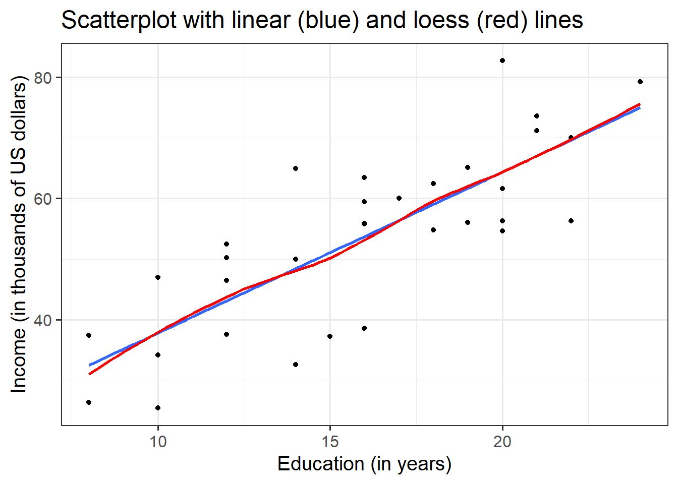
Check if the fitted model satisfies the linearity assumption for rv_mdl1.

Write a sentence summarising whether or not you consider the assumption to have been met. Justify your answer with reference to the plots.

Hint

Consider plotting residual vs fitted values, and/or a scatterplot with loess lines

Solution

As usual, there are multiple equivalent ways to check this. For a model with a single predictor, there are a couple of possibilities:

Residuals vs fitted values

#here what we need to see is that the red line is approximately horizontal at zero
plot(rv_mdl1, which = 1) 

The residuals appear to be randomly scattered around zero, without showing any pattern with respect to the fitted values. Thus, there is no sign of violation of the linearity assumption.

Scatterplots with loess lines

ggplot(rvdata, aes(x = education, y = income)) + 
    geom_point() + 
    geom_smooth(method = "lm", se=F) +
    geom_smooth(method = "loess", se=F, col = "red") +
    labs(x= "Education (in years)", y="Income (in thousands of US dollars)", title = "Scatterplot with linear (blue) and loess (red) lines")

From our scatterplot, the loess line closely follows the data. Hence, there is no sign of violation of the linearity assumption.

Question 3

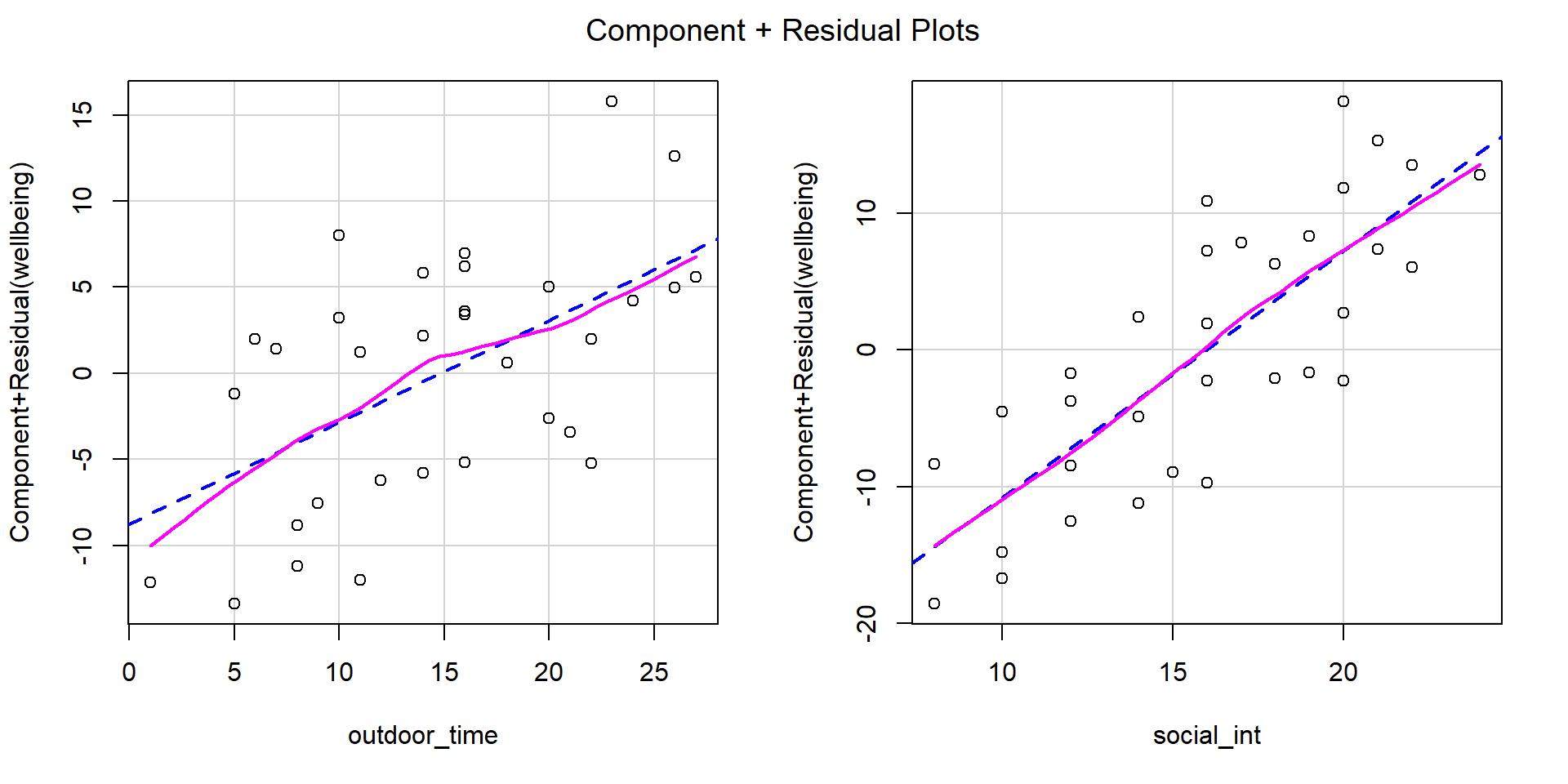
Check if the fitted model satisfies the linearity assumption for wb_mdl1.

Write a sentence summarising whether or not you consider the assumption to have been met. Justify your answer with reference to the plots.

Hint

When we have multiple predictors, we need to use component-residual plots (also known as partial-residual plots) to check the assumption of linearity.

Solution

crPlots(wb_mdl1)

The smoother (the pink line) follows quite closely to a linear relationship (the dashed blue line). This suggests that the linearity assumption is met.

Question 4

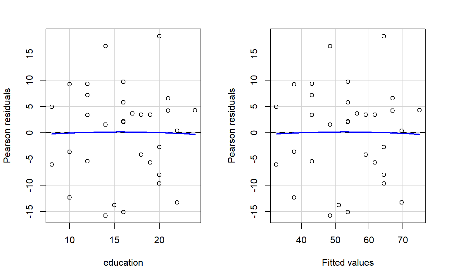
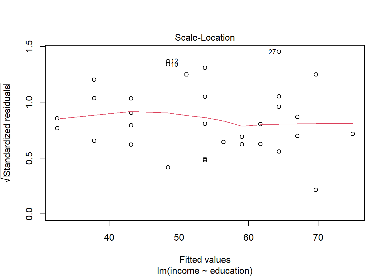
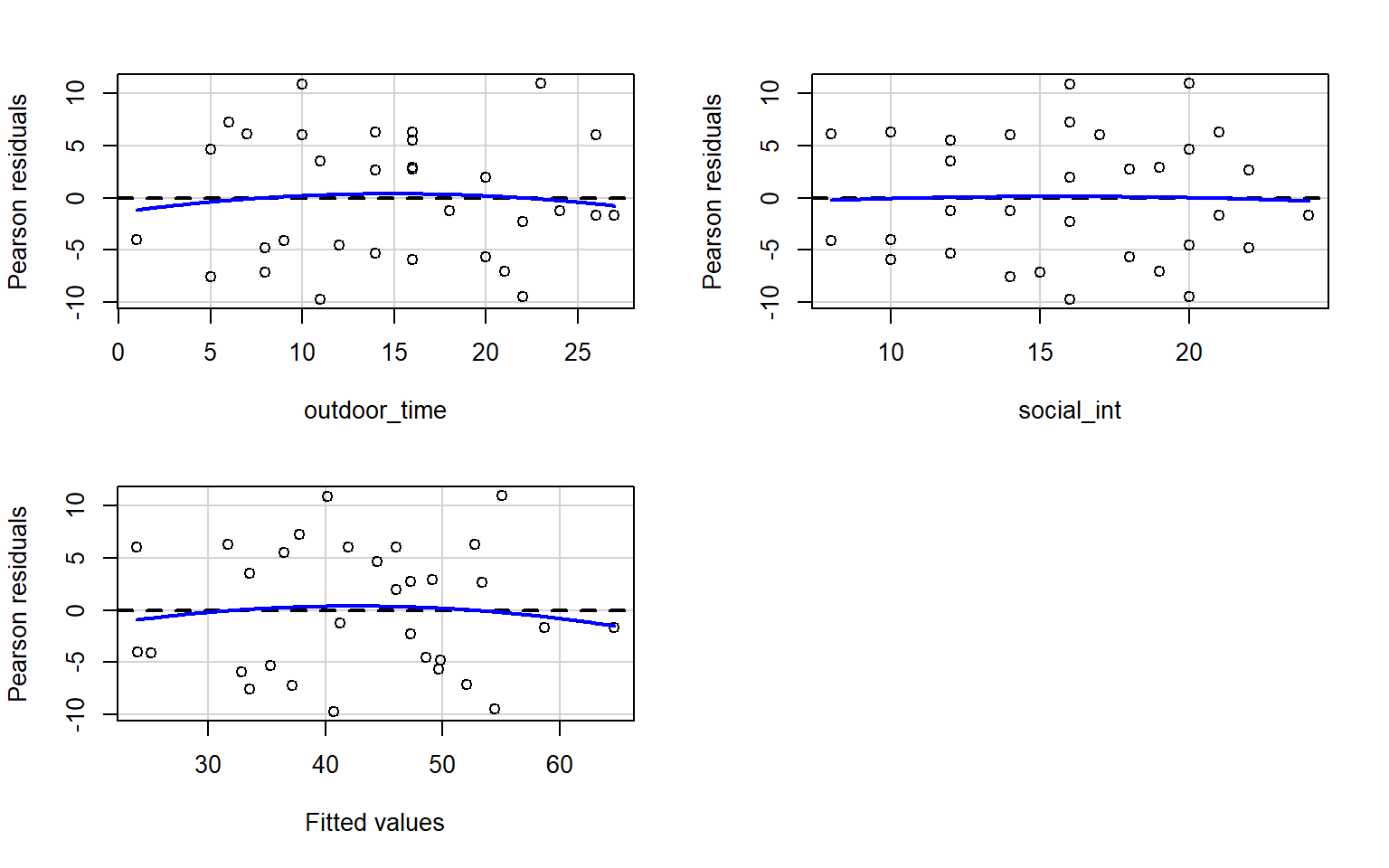
Check if the fitted models rv_mdl1 and wb_mdl1 satisfy the equal variance assumption.

Write a sentence summarising whether or not you consider the assumption to have been met for each model. Justify your answer with reference to plots.

Hint

Use residualPlots() to plot residuals against the predictor.

For interpretation - the vertical spread of the residuals should roughly be the same everywhere.

Solution

rv_mdl1 model

We can visually assess by plotting the Pearson residuals against the fitted values:

residualPlots(rv_mdl1)

           Test stat Pr(>|Test stat|)
education    -0.0744           0.9412
Tukey test   -0.0744           0.9407

Hint

Quick Tip

As the residuals can be positive or negative, we can make it easier to assess equal spread by improving the ‘resolution’ of the points.

We can make all residuals positive by discarding the sign (take the absolute value), and then take the square root to make them closer to each other.

A plot of \(\sqrt{|\text{Standardized residuals}|}\) against the fitted values is shown below:

plot(rv_mdl1, which = 3)

The plot above has the points closer to each other, and all above 0. The line seems to be relatively flat (as it should be if the spread was constant). The data met the assumption of equal variance.

The spread of the standardized residuals appears to be constant as the fitted values vary.

wb_mdl1 model

residualPlots(wb_mdl1)

             Test stat Pr(>|Test stat|)
outdoor_time   -0.3478           0.7306
social_int     -0.1068           0.9157
Tukey test     -0.4189           0.6753

Partial residual plots show no clear non-linear trends between residuals and predictors, hence there is little sign of non-constant variance. The data met the assumption of equal variance.

Question 5

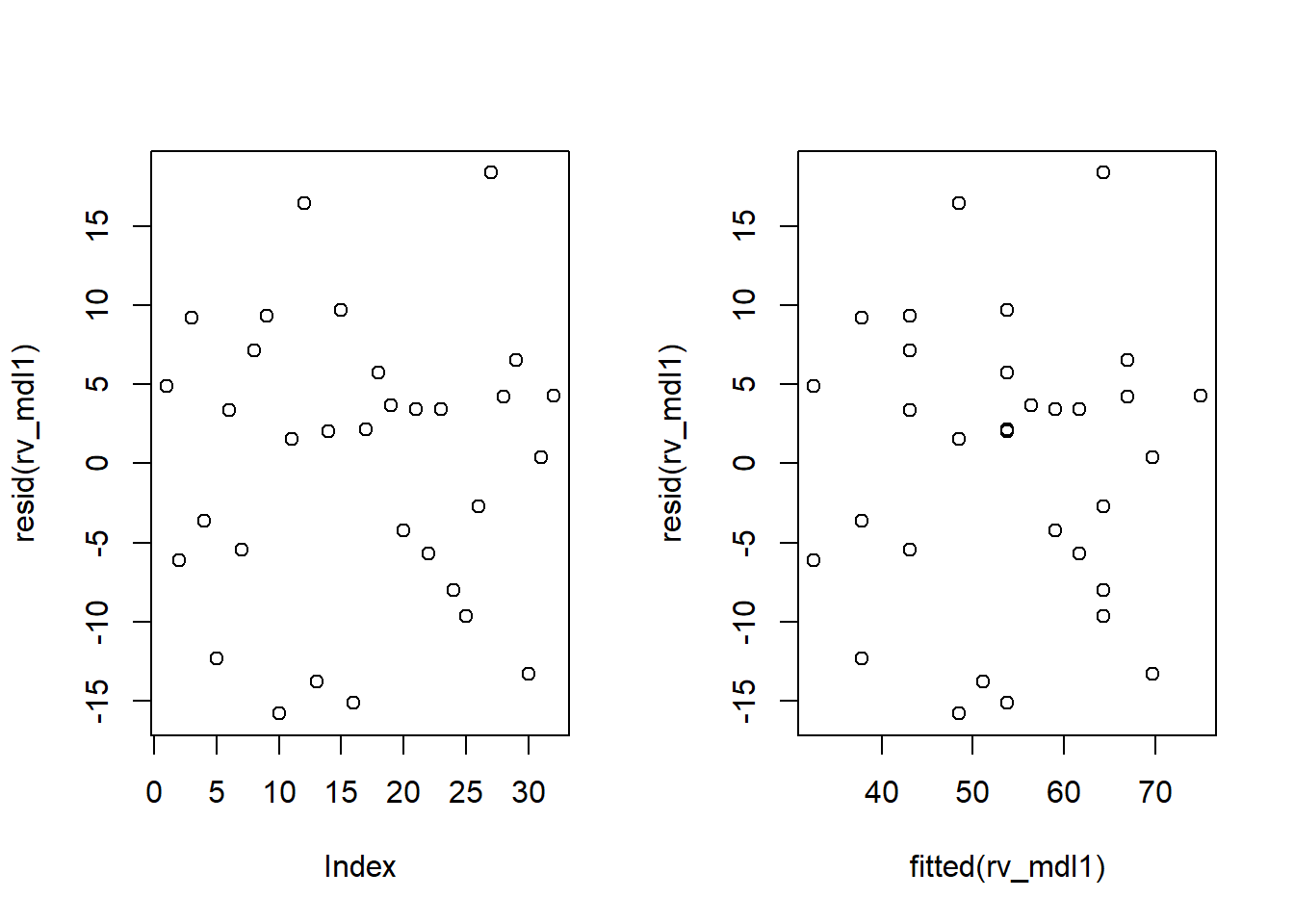
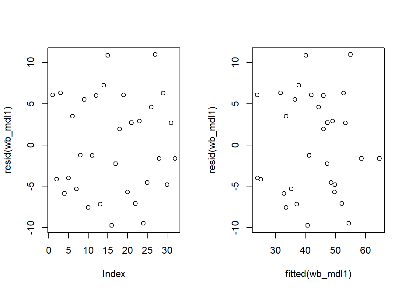
For both rv_mdl1 and wb_mdl1, visually assess whether there is autocorrelation in the error terms.

Write a sentence summarising whether or not you consider the assumption of independence to have been met for each (you may have to assume certain aspects of the study design).

Hint

To get a single figure made up of 2 by 1 panels, you can use the command par(mfrow = c(1,2)). Then create the plot. Then you need to go back to a single figure made up by a single panel with the command par(mfrow = c(1,1)).

Solution

rv_mdl1 model

par(mfrow = c(1,2))
plot(resid(rv_mdl1))
plot(fitted(rv_mdl1), resid(rv_mdl1))

par(mfrow = c(1,1))

Since our data were collected from a between-persons study design, we can assume the errors to be independent. This is supported by the plot of the residuals vs their index, as this shows no clear dependence (if they were collected over time, for example, and there was an increasing trend this would highlight a violation). The residuals vs fitted plot shows that there is no association between the errors and the model predictions.

wb_mdl1 model

par(mfrow = c(1,2))
plot(resid(wb_mdl1))
plot(fitted(wb_mdl1), resid(wb_mdl1))

par(mfrow = c(1,1))

Since our data were collected from a between-persons study design, we can assume the errors to be independent. This is supported by the plot of the residuals vs their index which shows no clear dependence, and the residuals vs fitted plot shows that there is no association between the errors and the model predictions.

Question 6

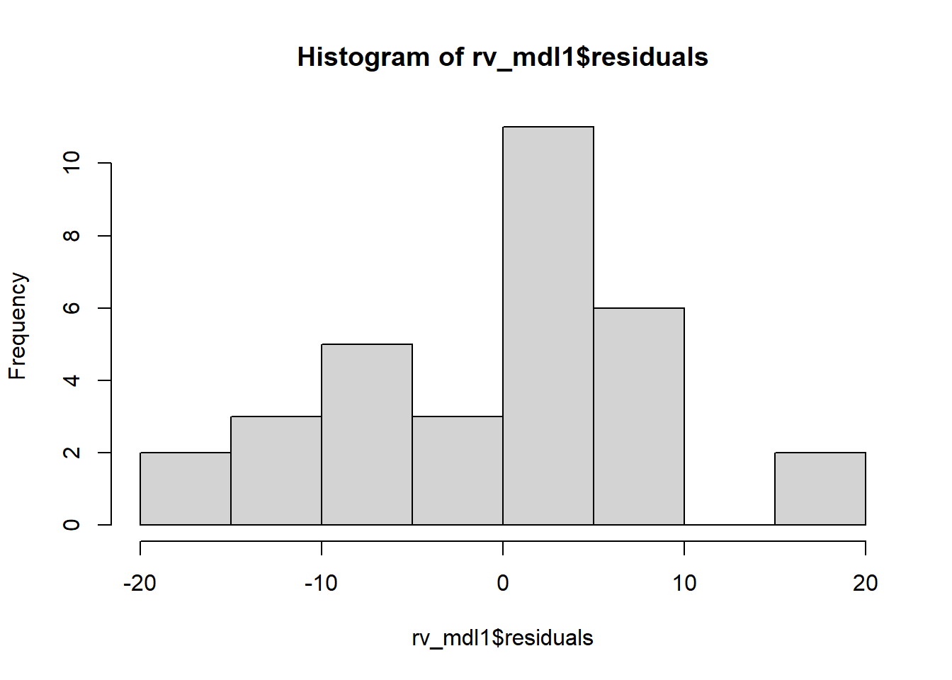
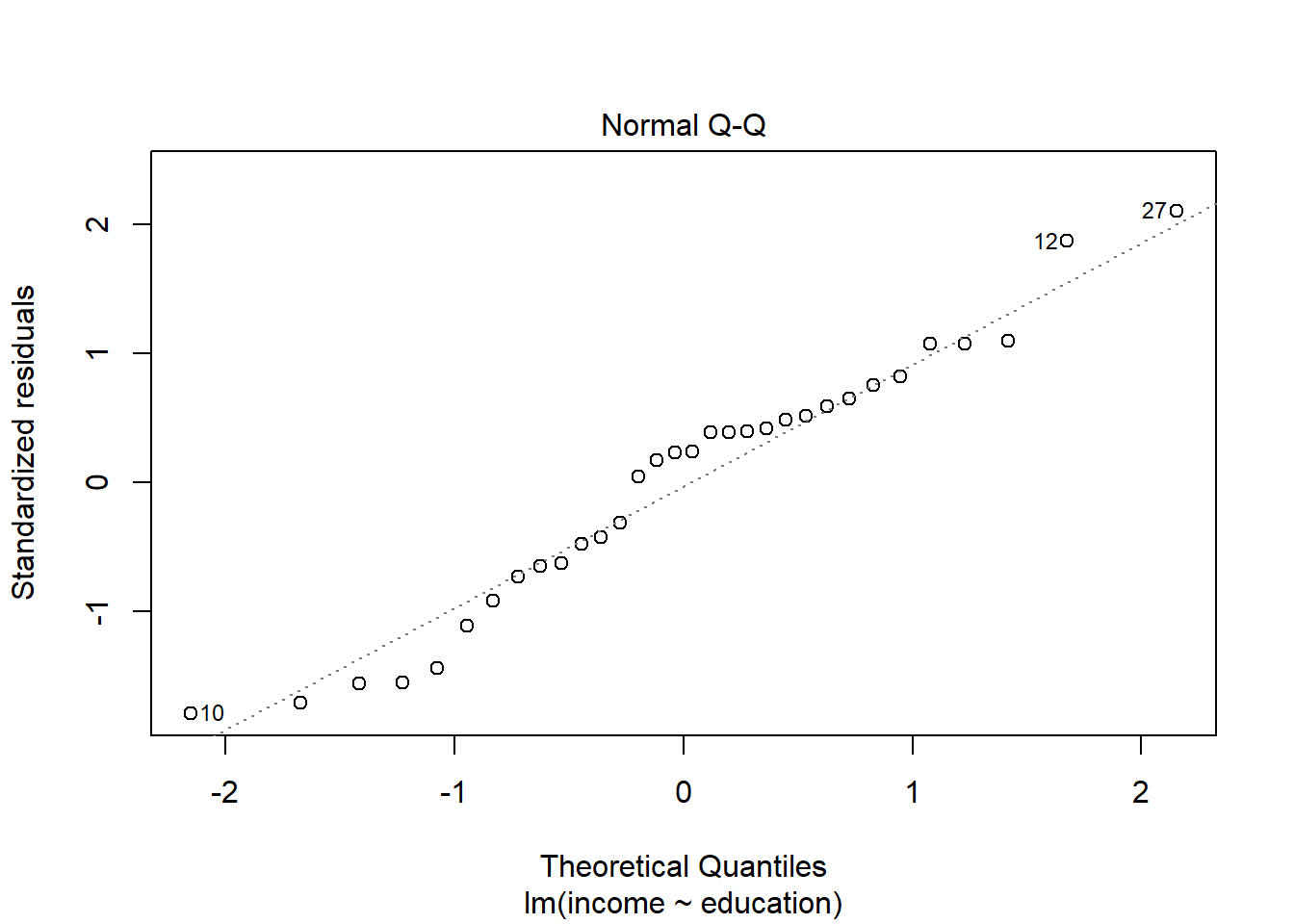
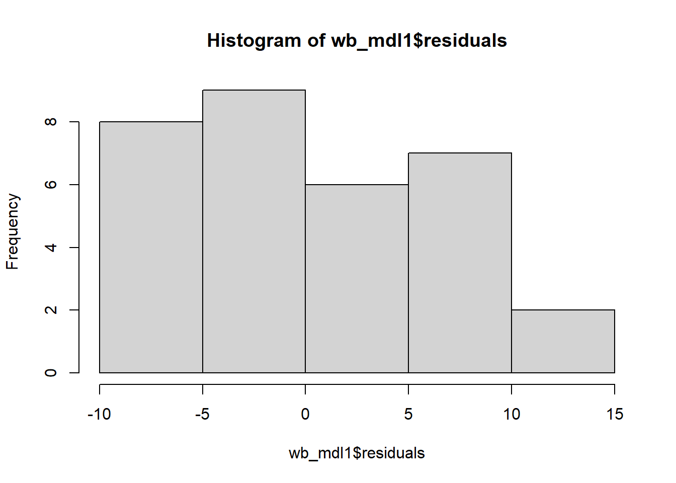
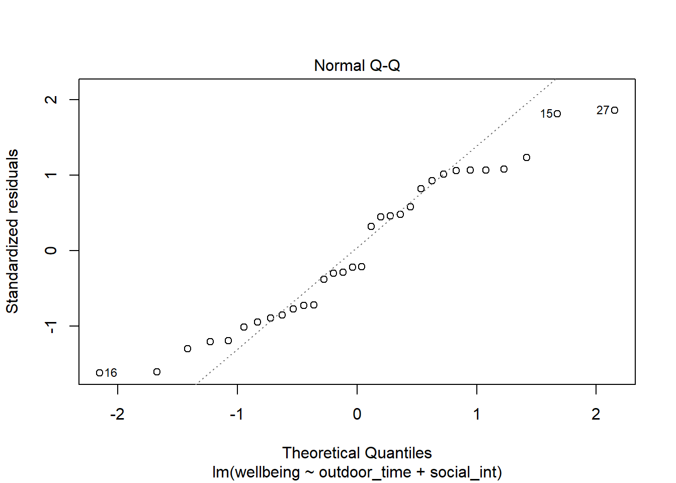
Check if the fitted models rv_mdl1 and wb_mdl1 satisfy the normality assumption.

Write a sentence summarising whether or not you consider the assumption to have been met. Justify your answer with reference to the plots.

Hint

We can get the QQplot from plot(model, which = ???), and you can plot the frequency distribution of the residuals via hist(model$residuals).

For interpretation - remember that departures from a linear trend in QQ plots indicate a lack of normality.

Solution

rv_mdl1 model

Histogram:

hist(rv_mdl1$residuals)

QQ Plot:

plot(rv_mdl1, which = 2)

The normal quantile plot follows a linear pattern and does not highlight any substantial skew or departure from normality.

wb_mdl1 model

Histogram:

hist(wb_mdl1$residuals)

QQ Plot:

plot(wb_mdl1, which = 2)

The QQplot indicated that the residuals follow close to a normal distribution. Although there is some evidence of heavier tails, given the small sample size (\(n\)=32) it is not of concern and we can be more conservative in our visual assessment of the plot.

For questions 7-10, we will be working with our wb_mdl1 only. Feel free to apply the below to your rv_mdl1 too as as extra practice during revision.

Multicollinearity

Question 7

For wb_mdl1, calculate the variance inflation factor (VIF) for the predictors in the model.

Write a sentence summarising whether or not you consider multicollinearity to be a problem here.

Solution

vif(wb_mdl1)

outdoor_time   social_int 
     1.13023      1.13023 

The VIF values for all predictors are <5, indicating that multicollinearity is not adversely affecting model estimates.

Diagnostics

Question 8

Create a new tibble which contains:

1. The original variables from the model (Hint, what does wb_mdl1$model give you?)
2. The fitted values from the model \(\hat y\)
   
3. The residuals \(\hat \epsilon\)
4. The studentised residuals
5. The hat values
6. The Cook’s Distance values

Solution

mdl_diagnost <- 
  tibble(
  wb_mdl1$model,
  fitted = fitted(wb_mdl1),
  resid = residuals(wb_mdl1),
  studres = rstudent(wb_mdl1),
  hats = hatvalues(wb_mdl1),
  cooksd = cooks.distance(wb_mdl1)
)

Question 9

From the tibble above, comment on the following:

• Looking at the studentised residuals, are there any outliers?
• Looking at the hat values, are there any observations with high leverage?
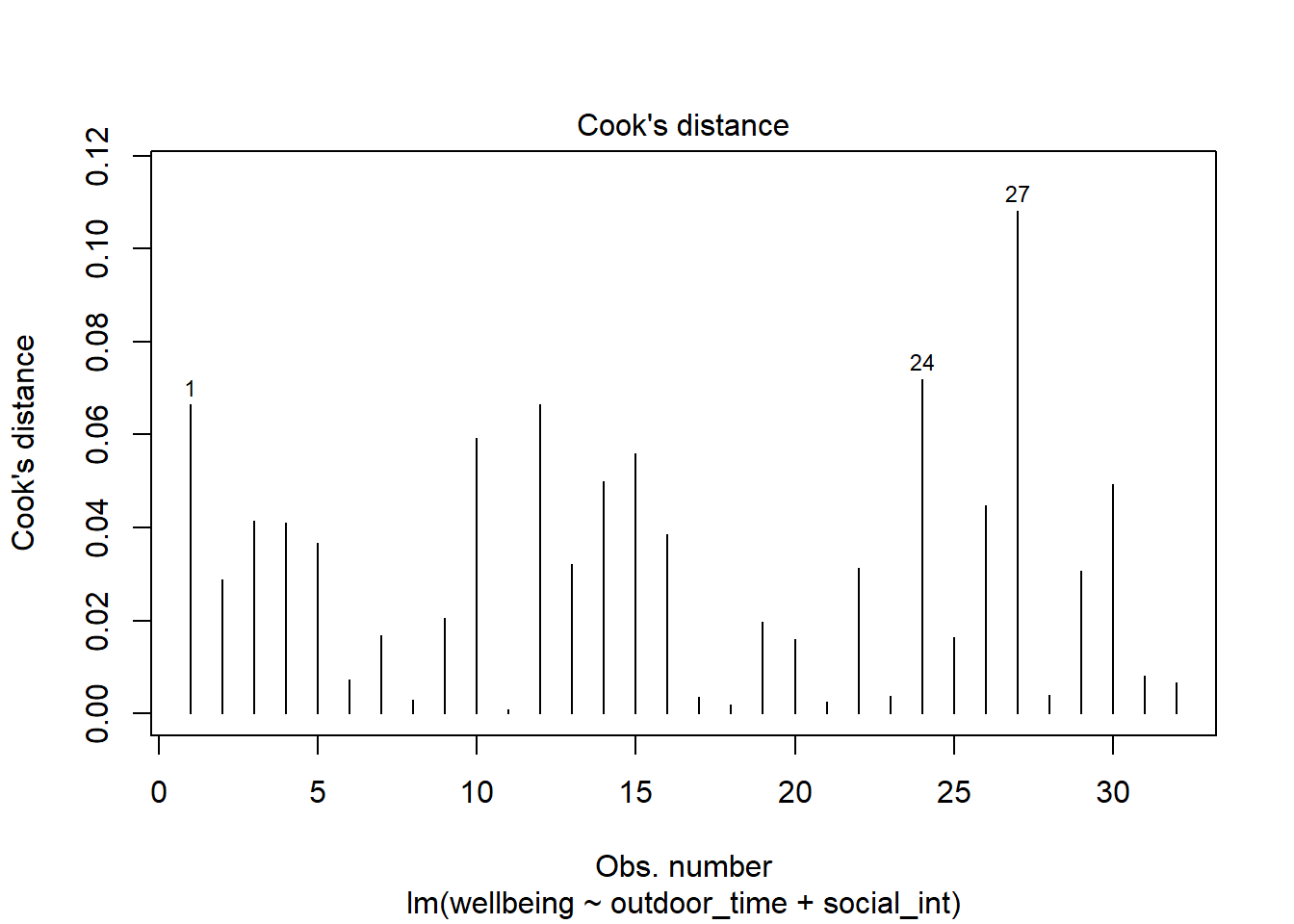
• Looking at the Cook’s Distance values, are there any highly influential points?

Solution

Outliers

In a standard normal distribution, 95% of the values are roughly between -2 and 2. Because of this, studentised residuals of \(>2\) or \(< -2\) indicate potential outlyingness.

We can ask R whether the absolute values (by specifying abs()) are \(>2\):

table(abs(mdl_diagnost$studres) > 2)

FALSE 
   32 

All values are FALSE, which tells us that none of the absolute values are \(>2\).

We could also filter our newly created tibble to these observations:

mdl_diagnost %>% 
  filter(abs(studres)>2)

# A tibble: 0 × 8
# … with 8 variables: wellbeing <dbl>, outdoor_time <dbl>, social_int <dbl>,
#   fitted <dbl>, resid <dbl>, studres <dbl>, hats <dbl>, cooksd <dbl>

There are zero rows in the tibble that have absolute values \(>2\).

There are no outliers in our data.

High Leverage

Recall that hat values of more than \(2 \bar{h}\) (2 times the average hat value) are considered high leverage. The average hat value, \(\bar{h}\) is calculated as \(\frac{k + 1}{n}\), where \(k\) is the number of predictors, and \(n\) is the sample size.

For our model: \[ \bar h = \frac{k+1}{n} = \frac{2+1}{32} = \frac{3}{32} = 0.094 \] We can ask whether any of observations have hat values which are greater than \(2 \bar h\):

mdl_diagnost %>%
  filter(hats > (2*0.094))

# A tibble: 0 × 8
# … with 8 variables: wellbeing <dbl>, outdoor_time <dbl>, social_int <dbl>,
#   fitted <dbl>, resid <dbl>, studres <dbl>, hats <dbl>, cooksd <dbl>

No values have been returned (the tibble has zero rows), hence we do not have any observations that have hat values which are greater than \(2 \bar h\).

There are 0 observations that have high leverage.

Influential Points

Recall that we have a Cook’s Distance cut-off of \(\frac{4}{n-k-1}\), where \(k\) is the number of predictors, and \(n\) is the sample size.

For our model: \[ D_{cutoff} = \frac{4}{n-k-1} = \frac{4}{32 - 2 - 1} = \frac{4}{29} = 0.138 \]

We can ask whether any of observations have a high influence on our model estimates:

mdl_diagnost %>%
  filter(cooksd > 0.138)

# A tibble: 0 × 8
# … with 8 variables: wellbeing <dbl>, outdoor_time <dbl>, social_int <dbl>,
#   fitted <dbl>, resid <dbl>, studres <dbl>, hats <dbl>, cooksd <dbl>

No values have been returned (the tibble has zero rows), hence we do not have any observations that have a high influence on our model estimates.

You can also display the Cook’s Distance values themselves using plot(model, which = 4):

plot(wb_mdl1, which = 4)

None of our observations have a high influence on our model estimates, as the maximum value of Cook’s distance in our sample is 0.108, which is less than the cutt-off value of 0.138. Thus, we do not appear to have any influential points in our sample.

Question 10

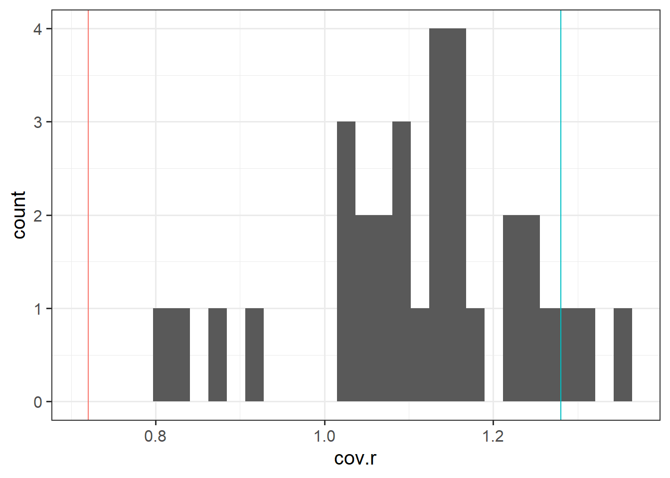
Use the function influence.measures() to extract these delete-1 measures of influence.

Try plotting the distributions of some of these measures.

Hint

The function influence.measures() returns an infl-type object. To plot this, we need to find a way to extract the actual numbers from it.
What do you think names(influence.measures(wb_mdl1)) shows you? How can we use influence.measures(wb_mdl1)$<insert name here> to extract the matrix of numbers?

Solution

inf_mes <- influence.measures(wb_mdl1)
round(inf_mes$infmat[1:10,],3)

   dfb.1_ dfb.otd_ dfb.scl_  dffit cov.r cook.d   hat
1   0.437   -0.111   -0.322  0.448 1.157  0.066 0.149
2  -0.282    0.032    0.230 -0.292 1.225  0.029 0.141
3   0.296    0.076   -0.290  0.354 1.088  0.042 0.097
4  -0.264   -0.131    0.293 -0.351 1.117  0.041 0.107
5  -0.271    0.227    0.105 -0.329 1.279  0.037 0.177
6   0.125   -0.027   -0.083  0.146 1.141  0.007 0.060
7  -0.174   -0.034    0.153 -0.223 1.087  0.017 0.060
8  -0.029   -0.073    0.061 -0.092 1.309  0.003 0.156
9   0.169    0.088   -0.178  0.248 1.088  0.021 0.067
10 -0.248    0.331   -0.006 -0.427 1.027  0.059 0.096

Let’s plot the distribution of COVRATIO statistics.

Recall that values which are \(>1+\frac{3(k+1)}{n}\) or \(<1-\frac{3(k+1)}{n}\) are considered as having strong influence.

For our model: \[ 1 \pm \frac{3(k+1)}{n} \quad = \quad 1 \pm\frac{3(2+1)}{32} \quad = \quad 1\pm \frac{9}{32} \quad = \quad 1\pm0.28 \] The “infmat” bit of an infl-type object contains the numbers, as we can see from out output above. To use it with ggplot, we will need to turn it into a dataframe (as.data.frame()), or a tibble (as_tibble()):

infdata <- inf_mes$infmat %>%
  as_tibble()

Now we can build our plot. It would be useful to add vertical lines at the values \(\quad 1\pm0.28\). To do so, we can use the geom_vline() function:

ggplot(data = infdata, aes(x = cov.r)) + 
  geom_histogram() +
  geom_vline(aes(xintercept = c(1-0.28), col = "blue")) +
  geom_vline(aes(xintercept = c(1+0.28), col = "red")) + 
  theme(legend.position = "none")  #remove legend

It looks like a few observations may be having quite a high influence here. This is perhaps not that surprising as we only have 32 datapoints.

© Copyright 2019-2022 The University of Edinburgh. Site licensed under the GNU AGPLv3 license.