Interactions III: Cat x Cat

Learning Objectives

At the end of this lab, you will:

1. Understand the concept of an interaction.
2. Be able to interpret a categorical \(\times\) categorical interaction.
3. Visualize and probe interactions.

What You Need

1. Be up to date with lectures
2. Have completed previous lab exercises from Week 7 and Week 8

Required R Packages

Remember to load all packages within a code chunk at the start of your RMarkdown file using library(). If you do not have a package and need to install, do so within the console using install.packages(" "). For further guidance on installing/updating packages, see Section C here.

For this lab, you will need to load the following package(s):

• tidyverse
• psych
• sjPlot
• kableExtra
• sandwich
• interactions

Lab Data

You can download the data required for this lab here or read it in via this link https://uoepsy.github.io/data/cognitive_experiment_3_by_2.csv

Study Overview

Research Question

Are there differences in types of memory deficits for those experiencing different cognitive impairment(s)?

A group of researchers wants to test a hypothesised theory according to which the difference in performance between explicit and implicit memory tasks will be greatest for Huntington patients in comparison to controls. On the other hand, the difference in performance between explicit and implicit memory tasks will not significantly differ between patients with amnesia in comparison to controls.

Cognitive Exp 3x2 data codebook.

Description

The researchers designed a study yielding a 3 by 2 factorial design to test this theory. The first factor, “Diagnosis”, classifies the three types of individuals:

• 1 denotes amnesic patients;
• 2 denotes Huntingtons patients; and
• 3 denotes a control group of individuals with no known neurological disorder.

The second factor, “Task”, tells us to which of two tasks each study participant was randomly assigned to:

• 1 = grammar task, which consists of classifying letter sequences as either following or not following grammatical rules; and
• 2 = recognition task, which consists of recognising particular stimuli as stimuli that have previously been presented during the task.

Keep in mind that each person has been randomly assigned to one of the two tasks, so there are five observations per cell of the design.¹

The tasks chosen by the researchers have been picked to map onto the theoretical differences between the three types of research participants. The first task (grammar) is known to reflect implicit memory processes, whereas the recognition task is known to reflect explicit memory processes. If the theory is correct, we would expect the difference in scores between the recognition and grammar tasks to be relatively similar for the control and amnesiac groups, but relatively larger for the Huntingtons group compared to controls.

Preview

The first ten rows of the data are:

Diagnosis	Task	Y
1	1	44
1	1	63
1	1	76
1	1	72
1	1	45
1	2	70

Setup

Setup

1. Create a new RMarkdown file
2. Load the required package(s)
3. Read the cognitive_experiment_3_by_2 dataset into R, assigning it to an object named cog

Solution

#Loading the required package(s)
library(tidyverse)
library(psych)
library(sjPlot)
library(kableExtra) 
library(sandwich)
library(interactions)

#Reading in data and storing in object named 'cog'
cog <- read_csv("https://uoepsy.github.io/data/cognitive_experiment_3_by_2.csv")

Exercises

Question 1

Examine the dataset, and perform any necessary and appropriate data management steps.

Hint

• Convert categorical variables to factors
• Label appropriately factors to aid with your model interpretations
• If needed, provide better variable names

Note that all of these steps can be done in combination - the mutate() and factor() functions will likely be useful here.

Solution

Let’s have a look at the data to see what we’re working with:

#first look at dataset structure
str(cog)

spc_tbl_ [30 × 3] (S3: spec_tbl_df/tbl_df/tbl/data.frame)
 $ Diagnosis: num [1:30] 1 1 1 1 1 1 1 1 1 1 ...
 $ Task     : num [1:30] 1 1 1 1 1 2 2 2 2 2 ...
 $ Y        : num [1:30] 44 63 76 72 45 70 51 82 66 56 ...
 - attr(*, "spec")=
  .. cols(
  ..   Diagnosis = col_double(),
  ..   Task = col_double(),
  ..   Y = col_double()
  .. )
 - attr(*, "problems")=<externalptr> 

#now lets look at top 6 rows (or the head) of the dataset
head(cog)

# A tibble: 6 × 3
  Diagnosis  Task     Y
      <dbl> <dbl> <dbl>
1         1     1    44
2         1     1    63
3         1     1    76
4         1     1    72
5         1     1    45
6         1     2    70

The columns Diagnosis and Task should be coded into factors with better labels, as currently, without making reference to the codebook, it is not clear what “1” and “2” represent. It is also unclear what the Y column represents - this should be renamed.

#We can make all of the changes noted above in one (long) command. 
#First we can use the function `factor()` by specifying the current levels and what labels each level should map to. 
#We can also simply rename the Y column to score. 

cog <- cog %>%
    mutate(
        Diagnosis = factor(Diagnosis, 
                           levels = c(1, 2, 3),
                           labels = c('Amnesic', 'Huntingtons', 'Control')),
        Task = factor(Task, 
                      levels = c(1, 2),
                      labels = c('Grammar', 'Recognition'))) %>%
    rename(Score = Y)

#Use head() function to check renaming
head(cog)

# A tibble: 6 × 3
  Diagnosis Task        Score
  <fct>     <fct>       <dbl>
1 Amnesic   Grammar        44
2 Amnesic   Grammar        63
3 Amnesic   Grammar        76
4 Amnesic   Grammar        72
5 Amnesic   Grammar        45
6 Amnesic   Recognition    70

Question 2

Choose appropriate reference levels for the Diagnosis and Task variables.

Solution

The Diagnosis factor has a group coded ‘Control’ which lends itself naturally to be the reference category.

cog$Diagnosis <- relevel(cog$Diagnosis, 'Control')

levels(cog$Diagnosis)

[1] "Control"     "Amnesic"     "Huntingtons"

There is no natural reference category for the Task factor, so we will leave it unaltered. However, if you are of a different opinion, please note that there is no absolute correct answer. As long as you interpret the model correctly, you will reach to the same conclusions as someone that has chosen a different baseline category.

Question 3

Formally state:

• a linear model to investigate whether there are differences in types of memory deficits for those experiencing different cognitive impairment(s)
• your chosen significance level
• the null and alternative hypotheses

Solution

Before stating the model, you first need to define the dummy variables for Diagnosis:

\[ D_\text{Amnesic} = \begin{cases} 1 & \text{if Diagnosis is Amnesic} \\ 0 & \text{otherwise} \end{cases} \quad D_\text{Huntingtons} = \begin{cases} 1 & \text{if Diagnosis is Huntingtons} \\ 0 & \text{otherwise} \end{cases} \quad (\text{Control is base level}) \]

And for Task:

\[ T_\text{Recognition} = \begin{cases} 1 & \text{if Task is Recognition} \\ 0 & \text{otherwise} \end{cases} \quad (\text{Grammar is base level}) \] The model becomes:

\[ \begin{aligned} Score &= \beta_0 \\ &+ \beta_1 D_\text{Amnesic} + \beta_2 D_\text{Huntingtons} \\ &+ \beta_3 T_\text{Recognition} \\ &+ \beta_4 (D_\text{Amnesic} * T_\text{Recognition}) + \beta_5 (D_\text{Huntingtons} * T_\text{Recognition}) \\ &+ \epsilon \end{aligned} \] Effects will be considered statistically significant at \(\alpha=.05\)

Our hypotheses are:

\(H_0: \beta_5 = 0\)

The difference in performance between explicit and implicit memory tasks does not significantly differ between patients with Huntingtons in comparison to Controls.

\(H_1: \beta_5 \neq 0\)

The difference in performance between explicit and implicit memory tasks does significantly differ between patients with Huntingtons in comparison to Controls.

Question 4

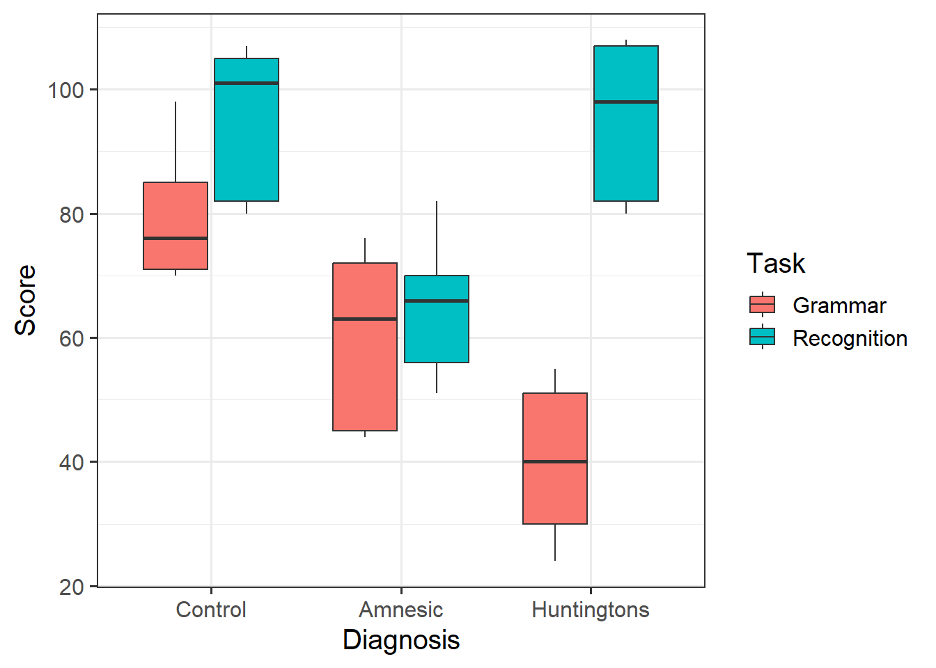
Provide a table of descriptive statistics and visualise your data.

Remember to interpret your plot in the context of the study.

Hint

1. For your table of descriptive statistics, both the group_by() and summarise() functions will come in handy here.
2. Recall that when visualising categorical variables, geom_boxplot() may be most appropriate to use.

Solution

First, lets look at our descriptive statistics and present in a well formatted table:

cog_desc <- cog %>% 
            group_by(Diagnosis, Task) %>%
            summarise(Mean = mean(Score),
                      SD = sd(Score),
                      Min = min(Score),
                      Max = max(Score)) %>% 
            kable(caption = "Descriptive Statistics", digits = 2) %>%
            kable_styling()

cog_desc

Table 1: Descriptive Statistics

Diagnosis	Task	Mean	SD	Min	Max
Control	Grammar	80	11.68	70	98
Control	Recognition	95	12.98	80	107
Amnesic	Grammar	60	14.92	44	76
Amnesic	Recognition	65	12.17	51	82
Huntingtons	Grammar	40	13.25	24	55
Huntingtons	Recognition	95	13.38	80	108

Next, look at associations among variables of interest:

cog_plt <- ggplot(cog, aes(x = Diagnosis, y = Score, fill = Task)) + 
  geom_boxplot() 
cog_plt

Figure 1: Associations among Score, Diagnosis, and Task

• Participants with Amnesia do not appear to differ in Score for Recognition or Grammar tasks. In comparison to Controls, Amnesic patients score lower on both tasks, but not considerably so.

• Participants with Huntingtons do differ in Score for Recognition and Grammar tasks, with higher scores on Recognition tasks. In comparison to Controls, Huntingtons patients score similarly on Recognition tasks, but considerably lower on Grammar tasks.

Question 5

Fit the specified model using lm(), and store the model in an object named “cog_mdl”.

Note

Fortunately, R computes the dummy variables for us! Thus. each row in the summary() output of the model will correspond to one of the estimated \(\beta\)’s in the equation above.

Solution

#fit interaction model
cog_mdl <- lm(Score ~ Diagnosis * Task, data = cog)

#check model output
summary(cog_mdl)

Call:
lm(formula = Score ~ Diagnosis * Task, data = cog)

Residuals:
   Min     1Q Median     3Q    Max 
-16.00 -12.25   2.00  11.75  18.00 

Coefficients:
                                     Estimate Std. Error t value Pr(>|t|)    
(Intercept)                            80.000      5.859  13.653 8.27e-13 ***
DiagnosisAmnesic                      -20.000      8.287  -2.414  0.02379 *  
DiagnosisHuntingtons                  -40.000      8.287  -4.827 6.45e-05 ***
TaskRecognition                        15.000      8.287   1.810  0.08281 .  
DiagnosisAmnesic:TaskRecognition      -10.000     11.719  -0.853  0.40192    
DiagnosisHuntingtons:TaskRecognition   40.000     11.719   3.413  0.00228 ** 
---
Signif. codes:  0 '***' 0.001 '**' 0.01 '*' 0.05 '.' 0.1 ' ' 1

Residual standard error: 13.1 on 24 degrees of freedom
Multiple R-squared:  0.7394,    Adjusted R-squared:  0.6851 
F-statistic: 13.62 on 5 and 24 DF,  p-value: 2.359e-06

Question 6

Recall your table of descriptive statistics - map each coefficient from the summary() output from “cog_mdl” to the group means.

Solution

cog_desc

Descriptive Statistics

Diagnosis	Task	Mean	SD	Min	Max
Control	Grammar	80	11.68	70	98
Control	Recognition	95	12.98	80	107
Amnesic	Grammar	60	14.92	44	76
Amnesic	Recognition	65	12.17	51	82
Huntingtons	Grammar	40	13.25	24	55
Huntingtons	Recognition	95	13.38	80	108

• \(\hat{\beta}_0\) = 80
  = Mean(Control, Grammar)

• \(\hat{\beta}_1\) = -20
  = Mean(Amnesic, Grammar) - Mean(Control, Grammar)
  = 60 - 80

• \(\hat{\beta}_2\) = -40
  = Mean(Huntingtons, Grammar) - Mean(Control, Grammar)
  = 40 - 80

• \(\hat{\beta}_3\) = 15
  = Mean(Control, Recognition) - Mean(Control, Grammar)
  = 95 - 80

• \(\hat{\beta}_4\) = -10
  = [Mean(Amnesic, Recognition) - Mean(Amnesic, Grammar)] -
  [Mean(Control, Recognition) - Mean(Control, Grammar)]
  = [65 - 60] - [95 - 80] = 5 - 15 = -10

• \(\hat{\beta}_5\) = 40
  = [Mean(Huntingtons, Recognition) - Mean(Huntingtons, Grammar)] -
  [Mean(Control, Recognition) - Mean(Control, Grammar)]
  = [95 - 40] - [95 - 80] = 55 - 15 = 40

Question 7

Interpret your coefficients in the context of the study.

Solution

Recall that we can obtain our parameter estimates using various functions such as summary(),coef(), coefficients(), etc.

coefficients(cog_mdl)

                         (Intercept)                     DiagnosisAmnesic 
                                  80                                  -20 
                DiagnosisHuntingtons                      TaskRecognition 
                                 -40                                   15 
    DiagnosisAmnesic:TaskRecognition DiagnosisHuntingtons:TaskRecognition 
                                 -10                                   40 

• \(\beta_0\) = (Intercept) = 80
  • The intercept, or predicted scores for those in the Control diagnosis condition on the Grammar task.
• \(\beta_1\) = DiagnosisAmnesic = -20
  • The difference in scores between Amnesic and Control conditions on the Grammar task
  • On the Grammar task, individuals with Amnesia scored 20 points lower than Control participants.
• \(\beta_2\) = DiagnosisHuntingtons = -40
  • The difference in score between Huntingtons and Control conditions on the Grammar task
  • On the Grammar task, individuals with Huntingtons scored 40 points lower than Control participants.
• \(\beta_3\) TaskRecognition = 15
  • The difference in score between individuals in the Control diagnosis condition completing Recognition and Grammar tasks.
  • Control participants scored 15 points higher when completing Recognition tasks in comparison to Grammar tasks.
• \(\beta_4\) DiagnosisAmnesic:TaskRecognition = -10
  • The difference between score in Amnesic and Control diagnosis conditions between Recognition and Grammar tasks.
  • The difference between Grammar and Recognition tasks is 10 points lower in the Amnesiac vs Control diagnosis conditions.
• \(\beta_5\) DiagnosisHuntingtons:TaskRecognition = 40
  • The difference between score in Huntingtons and Control diagnosis conditions between Recognition and Grammar tasks.
  • The difference between Grammar and Recognition tasks is 40 points higher in the Huntingtons vs Control diagnosis conditions.

Question 8

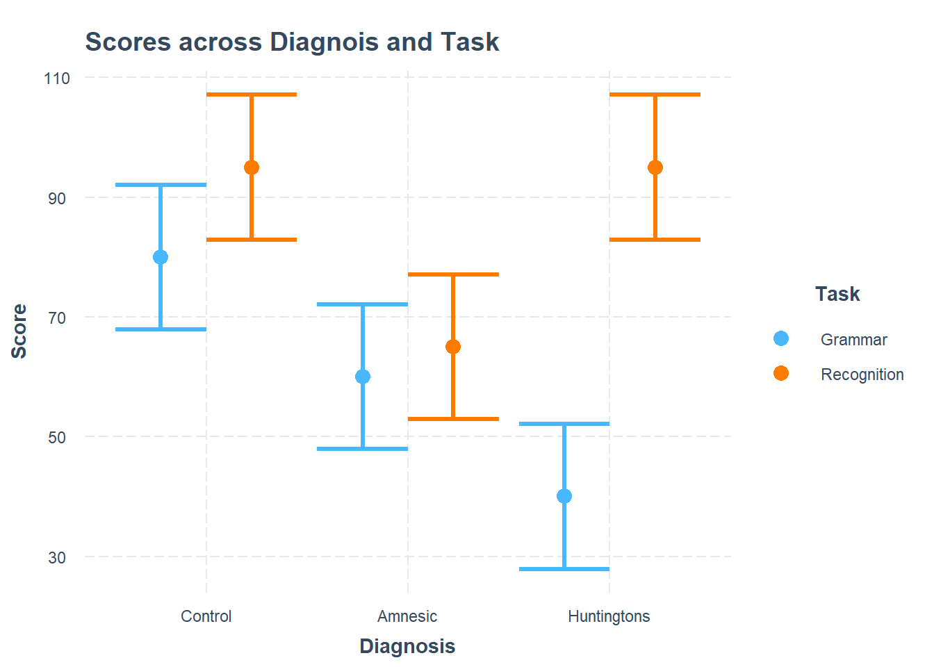
Using the cat_plot() function from the interactions package, visualise the interaction effects from your model.

Try to summarise the interaction effects in a few short and concise sentences.

Solution

plt_cog_mdl <- cat_plot(model = cog_mdl, 
                  pred = Diagnosis, 
                  modx = Task, 
                  main.title = "Scores across Diagnois and Task",
                  x.label = "Diagnosis",
                  y.label = "Score",
                  legend.main = "Task")
plt_cog_mdl

Figure 2: Interaction Plot

The effect of Task on Scores does appear to vary depending on Diagnosis.

The difference in score between recognition and grammar tasks for Huntingtons patients is larger than the difference in score between recognition and grammar tasks for the Control patients.

The difference in score between recognition and grammar tasks for Amnesic patients however does not appear to be very different (given the overlapping intervals) than the difference in score between recognition and grammar tasks for the Control patients.

How do we know there is an interaction?

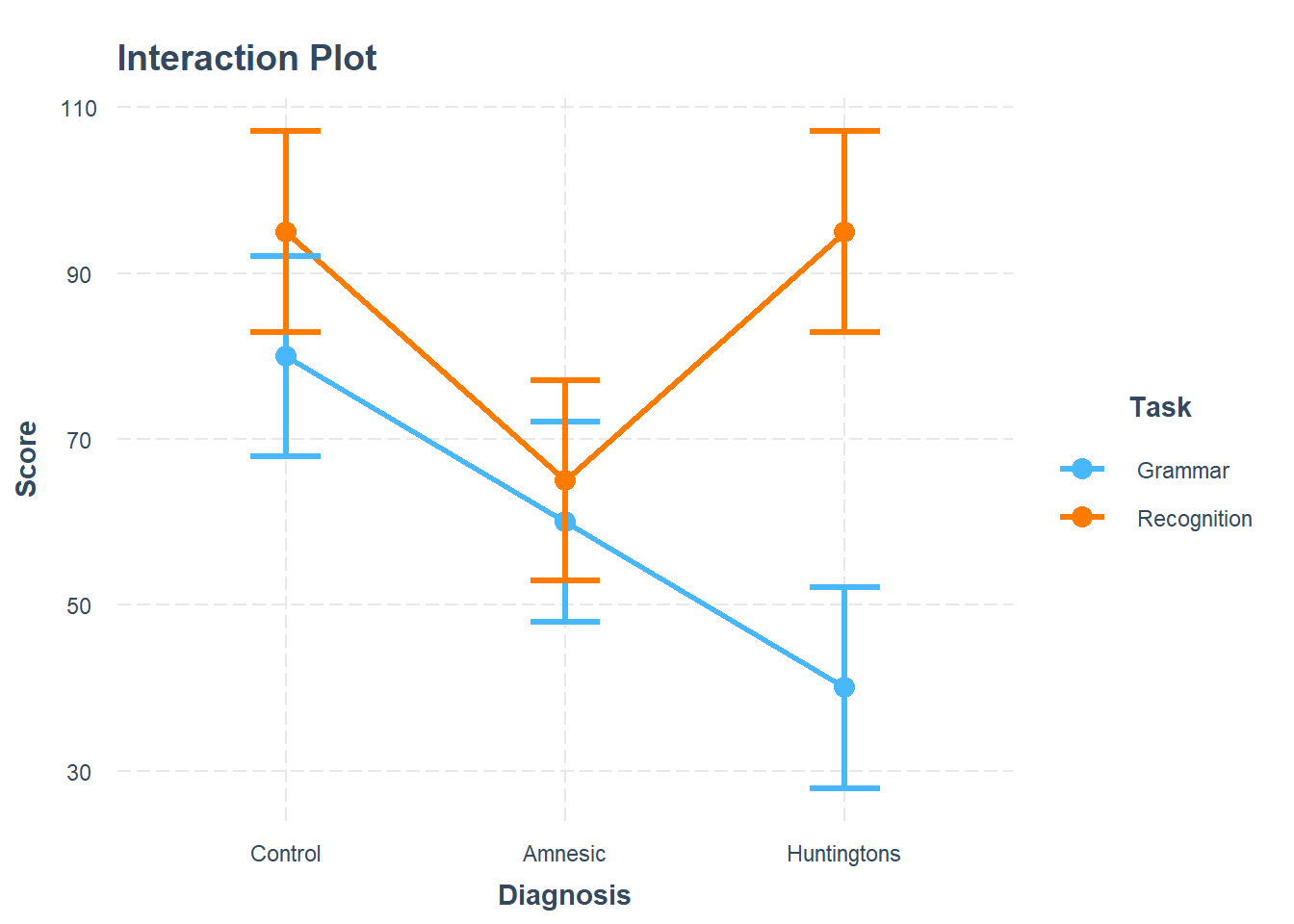
If you imagine connecting the dots of the same color with a line (you could specify geom = "line" in a new line in the code chunk above to do this), you can see that the two virtual lines are not parallel (see below plot), suggesting the presence of an interaction. The difference in score between recognition and grammar tasks for Huntingtons patients (consider the vertical difference) is larger than the difference in score between recognition and grammar tasks for the Control patients. If those vertical differences were the same, there would be no interaction.

Figure 3: Interaction Plot with Connected Lines

Question 9

Provide key model results in a formatted table.

Hint

Use tab_model() from the sjPlot package.

Remember that you can rename your DV and IV labels by specifying dv.labels and pred.labels.

Solution

#create table for results
tab_model(cog_mdl, 
          show.stat = TRUE,
          dv.labels = "Scores",
          title = "Regression table for Scores model")

Table 2: Regression table for Scores model

	Scores
Predictors	Estimates	CI	Statistic	p
(Intercept)	80.00	67.91 – 92.09	13.65	<0.001
Diagnosis [Amnesic]	-20.00	-37.10 – -2.90	-2.41	0.024
Diagnosis [Huntingtons]	-40.00	-57.10 – -22.90	-4.83	<0.001
Task [Recognition]	15.00	-2.10 – 32.10	1.81	0.083
Diagnosis [Amnesic] × Task [Recognition]	-10.00	-34.19 – 14.19	-0.85	0.402
Diagnosis [Huntingtons] × Task [Recognition]	40.00	15.81 – 64.19	3.41	0.002
Observations	30
R2 / R2 adjusted	0.739 / 0.685

Question 10

Interpret your results in the context of the research question and report your model in full.

Make reference to the interaction plot and regression table.

Solution

Full regression results including 95% Confidence Intervals are shown in Table 2. The \(F\)-test for model utility was significant \((F(5,24) = 13.62, p <.001)\), and the model explained approximately 68.5% of the variability in Scores.

The difference in scores between the recognition and grammar tasks, respectively measuring explicit and implicit memory, for amnesiac patients in comparison to controls was estimated to be -10 points, though this difference was not significantly different from zero \((t(24) = -0.85, p = .40)\).

The difference in scores between the recognition and grammar tasks, respectively measuring explicit and implicit memory, for Huntingtons patients in comparison to controls was significant, and indicated a difference of 40 points in explicit vs implicit memory performance \((t(24) = 3.41, p = .002)\). This interaction is visually presented in Figure 2.

Therefore, we have evidence to reject the null hypothesis (the difference in performance between explicit and implicit memory tasks does not significantly differ between patients with Huntingtons in comparison to Controls).

Footnotes

1. Some researchers may point out that a design where each person was assessed on both tasks might have been more efficient. However, the task factor in such design would then be within-subjects, meaning that the scores corresponding to the same person would be correlated. To analyse such design we will need a different method which is discussed next year!