Multiple Linear Regression

Learning Objectives

At the end of this lab, you will:

1. Extend the ideas of single linear regression to consider regression models with two or more predictors
2. Understand and interpret the coefficients in multiple linear regression models

Requirements

1. Be up to date with lectures
2. Have completed Week 1 and Week 2 lab exercises

Required R Packages

Remember to load all packages within a code chunk at the start of your RMarkdown file using library(). If you do not have a package and need to install, do so within the console using install.packages(" "). For further guidance on installing/updating packages, see Section C here.

For this lab, you will need to load the following package(s):

• tidyverse
• patchwork
• sjPlot

Lab Data

You can download the data required for this lab here or read it in via this link https://uoepsy.github.io/data/wellbeing.csv.

Setup

Setup

1. Create a new RMarkdown file
2. Load the required package(s)
3. Read the wellbeing dataset into R, assigning it to an object named mwdata

Solution

#Loading the required package(s)
library(tidyverse)
library(patchwork)
library(sjPlot)

# Reading in data and storing to an object named 'mwdata'
mwdata <- read_csv("https://uoepsy.github.io/data/wellbeing.csv")

Study Overview

Research Question

Is there an association between well-being and time spent outdoors after taking into account the association between well-being and social interactions?

Wellbeing data codebook.

Description

Researchers interviewed 32 participants, selected at random from the population of residents of Edinburgh & Lothians. They used the Warwick-Edinburgh Mental Wellbeing Scale (WEMWBS), a self-report measure of mental health and well-being. The scale is scored by summing responses to each item, with items answered on a 1 to 5 Likert scale. The minimum scale score is 14 and the maximum is 70.

The researchers also asked participants to estimate the average number of hours they spend outdoors each week, the average number of social interactions they have each week (whether on-line or in-person), and whether they believe that they stick to a routine throughout the week (Yes/No).

The data in wellbeing.csv contain five attributes collected from a random sample of \(n=32\) hypothetical residents over Edinburgh & Lothians, and include:

• wellbeing: Warwick-Edinburgh Mental Wellbeing Scale (WEMWBS), a self-report measure of mental health and well-being. The scale is scored by summing responses to each item, with items answered on a 1 to 5 Likert scale. The minimum scale score is 14 and the maximum is 70.
  
• outdoor_time: Self report estimated number of hours per week spent outdoors
  
• social_int: Self report estimated number of social interactions per week (both online and in-person)
• routine: Binary Yes/No response to the question “Do you follow a daily routine throughout the week?”
• location: Location of primary residence (City, Suburb, Rural)

Preview

The first six rows of the data are:

wellbeing	outdoor_time	social_int	location	routine
30	7	8	Suburb	Routine
21	9	8	City	No Routine
38	14	10	Suburb	Routine
27	16	10	City	No Routine
20	1	10	Rural	No Routine
37	11	12	Suburb	No Routine

Question 1

Produce plots of the marginal distributions (the distributions of each variable in the analysis without reference to the other variables) of the wellbeing, outdoor_time, and social_int variables.

Hint

• You could use, for example, geom_density() for a density plot or geom_histogram() for a histogram.
• Look at the shape, center and spread of the distribution. Is it symmetric or skewed? Is it unimodal or bimodal?

Solution

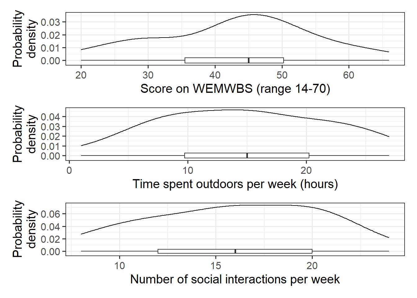
We should be familiar now with how to visualise a marginal distribution. You might choose histograms, density curves, or boxplots, or a combination:

wellbeing_plot <- 
  ggplot(data = mwdata, aes(x = wellbeing)) +
  geom_density() +
  geom_boxplot(width = 1/250) +
  labs(x = "Score on WEMWBS (range 14-70)", y = "Probability\ndensity")

outdoortime_plot <- 
  ggplot(data = mwdata, aes(x = outdoor_time)) +
  geom_density() +
  geom_boxplot(width = 1/200) +
  labs(x = "Time spent outdoors per week (hours)", y = "Probability\ndensity")

social_plot <- 
  ggplot(data = mwdata, aes(x = social_int)) +
  geom_density() +
  geom_boxplot(width = 1/150) +
  labs(x = "Number of social interactions per week", y = "Probability\ndensity")

# the "patchwork" library allows us to arrange multiple plots
wellbeing_plot / outdoortime_plot / social_plot

Figure 1: Marginal distribution plots of wellbeing sores, weekly hours spent outdoors, and social interactions

Summary statistics for wellbeing, outdoor time, and social interactions:

descriptives <- mwdata %>% 
  summarize(
    M_Wellbeing = mean(wellbeing), 
    SD_Wellbeing = sd(wellbeing),
    M_OutTime = mean(outdoor_time), 
    SD_OutTime = sd(outdoor_time),
    M_SocInt = mean(social_int), 
    SD_SocInt = sd(social_int)
    )
descriptives

# A tibble: 1 × 6
  M_Wellbeing SD_Wellbeing M_OutTime SD_OutTime M_SocInt SD_SocInt
        <dbl>        <dbl>     <dbl>      <dbl>    <dbl>     <dbl>
1          43         11.7      14.8       6.95       16      4.36

• The marginal distribution of scores on the WEMWBS is unimodal with a mean of approximately 43. There is variation in WEMWBS scores (SD = 11.7).
  
• The marginal distribution of weekly hours spent outdoors is unimodal with a mean of approximately 14.8. There is variation in weekly hours spent outdoors (SD = 6.9).
  
• The marginal distribution of numbers of social interactions per week is unimodal with a mean of approximately 16. There is variation in numbers of social interactions (SD = 4.4).

Question 2

Produce plots of the associations between the outcome variable (wellbeing) and each of the explanatory variables.

Hint

Think about:

• Direction of association
• Form of association (can it be summarised well with a straight line?)
  
• Strength of association (how closely do points fall to a recognizable pattern such as a line?)
• Unusual observations that do not fit the pattern of the rest of the observations and which are worth examining in more detail.

Plot tips:

• use \n to wrap text in your titles and or axis labels
• consider using geom_smooth() to superimpose the best-fitting line describing the association of interest

Solution

wellbeing_outdoor <- 
  ggplot(data = mwdata, aes(x = outdoor_time, y = wellbeing)) +
  geom_point(alpha = 0.5) +
  geom_smooth(method = "lm", se = FALSE) + 
  labs(x = "Time spent outdoors \nper week (hours)", y = "Wellbeing score (WEMWBS)")

wellbeing_social <- 
  ggplot(data = mwdata, aes(x = social_int, y = wellbeing)) +
  geom_point(alpha = 0.5) +
  geom_smooth(method = "lm", se = FALSE) + 
  labs(x = "Number of social interactions \nper week", y = "Wellbeing score (WEMWBS)")

# place plots adjacent to one another
wellbeing_outdoor | wellbeing_social

Figure 2: Scatterplots displaying the relationships between scores on the WEMWBS and a) weekly outdoor time (hours), and b) weekly number of social interactions

Question 3

Produce a correlation matrix of the variables which are to be used in the analysis, and write a short paragraph describing the associations.

Correlation matrix

A table showing the correlation coefficients - \(r_{(x,y)}=\frac{\mathrm{cov}(x,y)}{s_xs_y}\) - between variables. Each cell in the table shows the relationship between two variables. The diagonals show the correlation of a variable with itself (and are therefore always equal to 1).

In R, we can create a correlation matrix by giving the cor() function a dataframe. However, we only want to give it 3 columns here. Think about how we select specific columns, either using select(), or giving the column numbers inside [].

Hint

Make sure to round your numbers in-line with APA 7th edition guidelines. The round() function will come in handy here, as might this APA numbers and statistics guide!

Solution

We can either use:

# correlation matrix of the first 3 columns
round(cor(mwdata[,1:3]), digits = 2)

or:

# select only the columns we want by name, and pass this to cor()
mwdata %>% 
  select(wellbeing, outdoor_time, social_int) %>%
  cor() %>%
    round(digits = 2)

             wellbeing outdoor_time social_int
wellbeing         1.00         0.58       0.79
outdoor_time      0.58         1.00       0.34
social_int        0.79         0.34       1.00

• There was a moderate, positive, linear association between weekly outdoor time and WEMWBS scores for the participants in the sample (\(r\) = .58). Higher number of hours spent outdoors each week was associated, on average, with higher wellbeing scores,
  
• There was a moderate, positive, linear association between the weekly number of social interactions and WEMWBS scores for the participants in the sample (\(r\) = .79). More social interactions were associated, on average, with higher wellbeing scores.
• There was a weak positive correlation between weekly outdoor time and the weekly number of social interactions (\(r\) = .34).

Note

Note that there is a weak correlation between our two explanatory variables (outdoor_time and social_int). We will return to how this might affect our model when later on we look at the assumptions of multiple regression.

Question 4

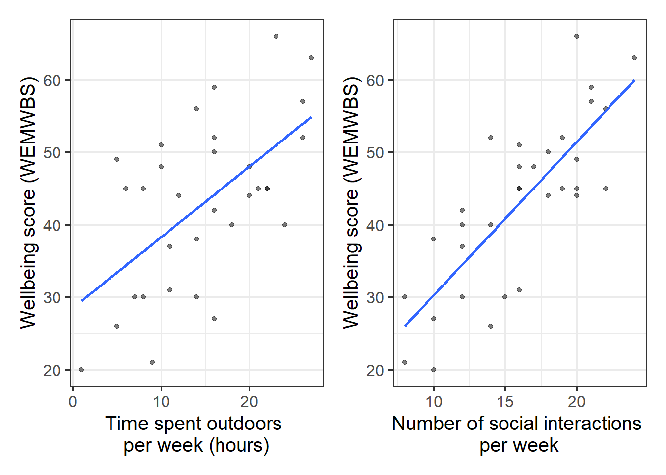
The scatterplots we created above show moderate, positive, and linear relationships both between outdoor time and wellbeing, and between numbers of social interactions and wellbeing.

1. Specify the form of your model, where \(y\) = scores on the WEMWBS, \(x_1\) = weekly number of social interactions, and \(x_2\) = weekly outdoor time.

2. What are the parameters of the model. How do we denote parameter estimates?

3. Fit the linear model in using lm(), assigning the output to an object called mdl1.

Hint

As we did for simple linear regression, we can fit our multiple regression model using the lm() function. We can add as many explanatory variables as we like, separating them with a +.

( <response variable> ~ 1 + <explanatory variable 1> + <explanatory variable 2> + ... , data = <dataframe> )

Solution

A model for the relationship between \(x_1\) = weekly outdoor time, \(x_2\) = weekly numbers of social interactions and \(y\) = scores on the WEMWBS is given by: \[ y = \beta_0 + \beta_1 x_1 + \beta_2 x_2 + \epsilon \\ \quad \\ \text{where} \quad \epsilon \sim N(0, \sigma) \text{ independently} \]

In the model specified above,

• \(\mu_{y|x_1, x_2} = \beta_0 + \beta_1 x + \beta_2 x_2\) represents the systematic part of the model giving the mean of \(y\) at each combination of values of \(x_1\) and \(x_2\);
• \(\epsilon\) represents the error (deviation) from that mean, and the errors are independent from one another.

The parameters of our model are:

• \(\beta_0\) (The intercept);
• \(\beta_1\) (The slope across values of \(x_1\));
• \(\beta_2\) (The slope across values of \(x_2\));
  
• \(\sigma\) (The standard deviation of the errors).

When we estimate these parameters from the available data, we have a fitted model (recall that the h\(\hat{\textrm{a}}\)ts are used to distinguish our estimates from the true unknown parameters): \[ \widehat{Wellbeing} = \hat \beta_0 + \hat \beta_1 \cdot Social Interactions + \hat \beta_2 \cdot Outdoor Time \] And we have residuals \(\hat \epsilon = y - \hat y\) which are the deviations from the observed values and our model-predicted responses.

Fitting the model in R:

mdl1 <- lm(wellbeing ~ social_int + outdoor_time, data = mwdata)

Visual

Note that for simple linear regression we talked about our model as a line in 2 dimensions: the systematic part \(\beta_0 + \beta_1 x\) defined a line for \(\mu_y\) across the possible values of \(x\), with \(\epsilon\) as the random deviations from that line. But in multiple regression we have more than two variables making up our model.

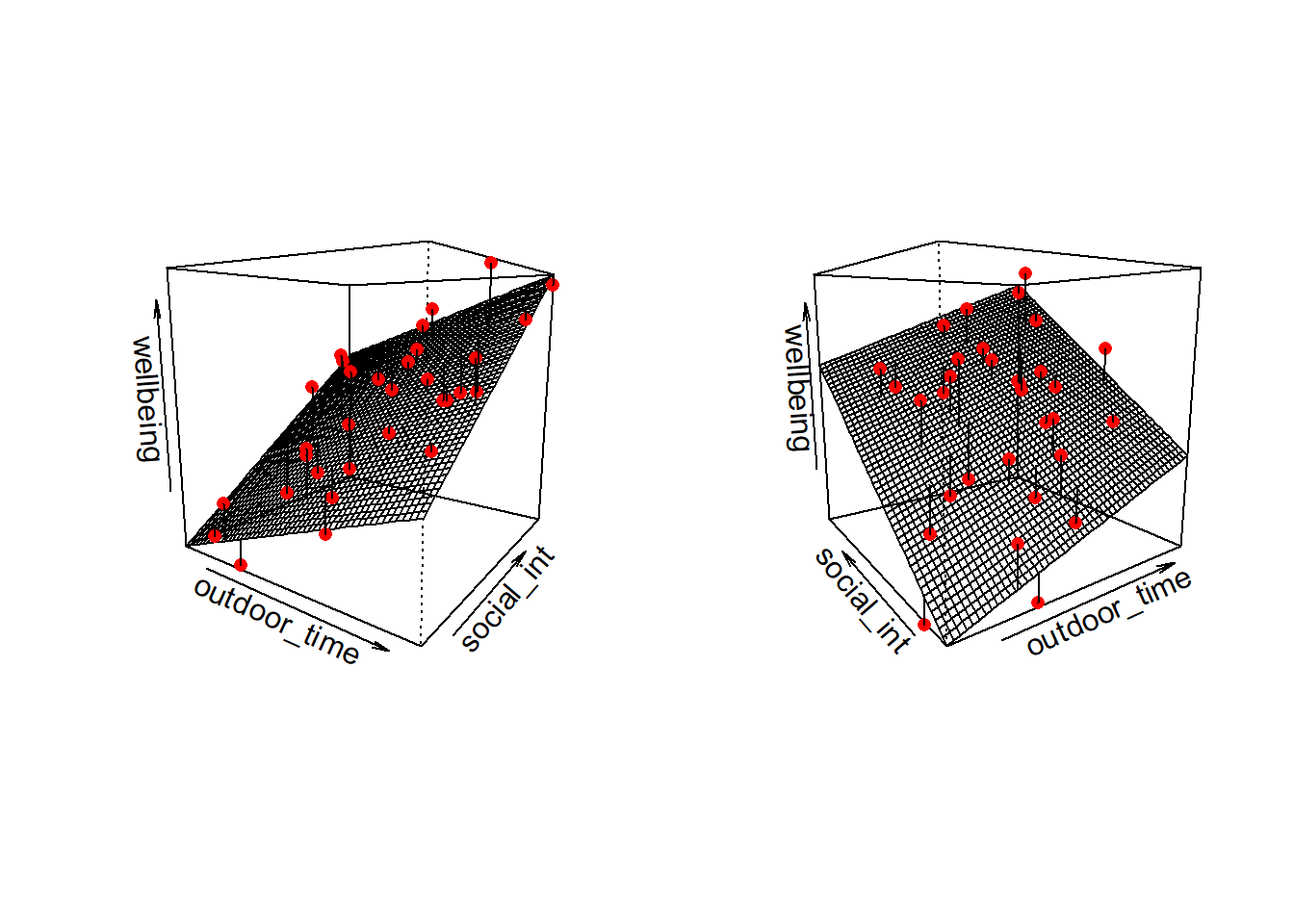
In this particular case of three variables (one outcome + two explanatory), we can think of our model as a regression surface (see Figure 3). The systematic part of our model defines the surface across a range of possible values of both \(x_1\) and \(x_2\). Deviations from the surface are determined by the random error component, \(\hat \epsilon\).

Figure 3: Regression surface for wellbeing ~ social_int + outdoor_time, from two different angles

Don’t worry about trying to figure out how to visualise it if we had any more explanatory variables! We can only concieve of 3 spatial dimensions. One could imagine this surface changing over time, which would bring in a 4th dimension, but beyond that, it’s not worth trying!.

Question 5

State the research question in the form of a testable hypothesis.

Hint

You must define both a null (\(H_0\)) and alternative hypothesis (\(H_1\)).

Solution

In words:

\(H_0\): There is no association between well-being and time spent outdoors after taking into account the relationship between well-being and social interactions

\(H_1\): There is an association between well-being and time spent outdoors after taking into account the relationship between well-being and social interactions

In symbols:

\(H_0: \beta_2 = 0\)

\(H_1: \beta_2 \neq 0\)

Question 6

Using any of:

• mdl1
• mdl1$coefficients
• coef(mdl1)
• coefficients(mdl1)
• summary(mdl1)

Write out the estimated parameter values of:

1. \(\hat \beta_0\), the estimated average wellbeing score associated with zero hours of outdoor time and zero social interactions per week.
   
2. \(\hat \beta_1\), the estimated increase in average wellbeing score associated with an additional social interaction per week (an increase of one), holding weekly outdoor time constant.
   
3. \(\hat \beta_2\), the estimated increase in average wellbeing score associated with one hour increase in weekly outdoor time, holding the number of social interactions constant

Note

Q: What do we mean by hold constant / controlling for / partialling out / residualizing for?

A: When the remaining explanatory variables are held at the same value or are fixed.

Solution

mdl1$coefficients

mdl1$coefficients

 (Intercept)   social_int outdoor_time 
   5.3703775    1.8034489    0.5923673 

coef(mdl1)

coef(mdl1)

 (Intercept)   social_int outdoor_time 
   5.3703775    1.8034489    0.5923673 

coefficients(mdl1)

coefficients(mdl1)

 (Intercept)   social_int outdoor_time 
   5.3703775    1.8034489    0.5923673 

summary(mdl1)

Look under the “Estimate” column:

summary(mdl1)

Call:
lm(formula = wellbeing ~ social_int + outdoor_time, data = mwdata)

Residuals:
   Min     1Q Median     3Q    Max 
-9.742 -4.915 -1.255  5.628 10.936 

Coefficients:
             Estimate Std. Error t value Pr(>|t|)    
(Intercept)    5.3704     4.3205   1.243   0.2238    
social_int     1.8034     0.2691   6.702 2.37e-07 ***
outdoor_time   0.5924     0.1689   3.506   0.0015 ** 
---
Signif. codes:  0 '***' 0.001 '**' 0.01 '*' 0.05 '.' 0.1 ' ' 1

Residual standard error: 6.148 on 29 degrees of freedom
Multiple R-squared:  0.7404,    Adjusted R-squared:  0.7224 
F-statistic: 41.34 on 2 and 29 DF,  p-value: 3.226e-09

1. \(\hat \beta_0\) = 5.37
   
2. \(\hat \beta_1\) = 1.8
   
3. \(\hat \beta_2\) = 0.59

Question 7

Within what distance from the model predicted values (the regression surface) would we expect 95% of wEMWBS wellbeing scores to be?

Hint

Either sigma() or part of the output from summary() will help you here.

Solution

sigma(mdl1)

sigma(mdl1)

[1] 6.148276

summary(mdl1)

Look at the “Residual standard error” entry of the summary(mdl) output:

summary(mdl1)

Call:
lm(formula = wellbeing ~ social_int + outdoor_time, data = mwdata)

Residuals:
   Min     1Q Median     3Q    Max 
-9.742 -4.915 -1.255  5.628 10.936 

Coefficients:
             Estimate Std. Error t value Pr(>|t|)    
(Intercept)    5.3704     4.3205   1.243   0.2238    
social_int     1.8034     0.2691   6.702 2.37e-07 ***
outdoor_time   0.5924     0.1689   3.506   0.0015 ** 
---
Signif. codes:  0 '***' 0.001 '**' 0.01 '*' 0.05 '.' 0.1 ' ' 1

Residual standard error: 6.148 on 29 degrees of freedom
Multiple R-squared:  0.7404,    Adjusted R-squared:  0.7224 
F-statistic: 41.34 on 2 and 29 DF,  p-value: 3.226e-09

The estimated standard deviation of the errors is \(\hat \sigma\) = 6.15. We would expect 95% of wellbeing scores to be within about 12.3 (\(2 \hat \sigma\)) from the model fit.

Question 8

Based on the model, predict the wellbeing scores for the following individuals:

• Leah: Social Interactions = 24; Outdoor Time = 3
• Sean: Social Interactions = 19; Outdoor Time = 26
• Mike: Social Interactions = 15; Outdoor Time = 20
• Donna: Social Interactions = 7; Outdoor Time = 2

Who has the highest predicted wellbeing score, and who has the lowest?

Solution

First we need to pass the data into R:

wellbeing_query <- tibble(social_int = c(24, 19, 15, 7),
                          outdoor_time = c(3, 26, 20, 2))

And next use predict() to get their estimated wellbeing scores:

predict(mdl1, newdata = wellbeing_query)

       1        2        3        4 
50.43025 55.03746 44.26946 19.17925 

Sean has the highest predicted wellbeing score (55.04), and Donna the lowest (19.18).

Question 9

Should we reject or fail to reject \(H_0\)? Why?

Solution

The research question asked whether there was an association between well-being and time spent outdoors after taking into account the association between well-being and social interactions. This was equivalent to testing the following null hypothesis:

\(H_0: \beta_2 = 0\)

Based on the model output (if we considered effects to be significant at \(\alpha\) = .05), we should reject the null hypothesis since our \(p\)-value smaller than this (\(p\) = .0015). In short, we reject the null since \(p\) < .05.

Question 10

Interpret the outdoor time coefficient in the context of the research question.

Solution

A multiple regression model was used to determine if there was an association between well-being and time spent outdoors after taking into account the association between well-being and social interactions. Outdoor time was significantly associated with wellbeing scores (\(\beta\) = 0.59, SE = 0.17, \(p\) < .001) after controlling for the number of weekly social interactions. Results suggested that for every additional hour spent outdoors each week, wellbeing scores increased by 0.59 points.