Binary Logistic Regression

Learning Objectives

At the end of this lab, you will:

1. Understand when to use a logistic model
2. Understand how to fit and interpret a logistic model

What You Need

1. Be up to date with lectures
2. Have completed Labs 1-5

Required R Packages

Remember to load all packages within a code chunk at the start of your RMarkdown file using library(). If you do not have a package and need to install, do so within the console using install.packages(" "). For further guidance on installing/updating packages, see Section C here.

For this lab, you will need to load the following package(s):

• tidyverse
• patchwork
• kableExtra
• psych
• sjPlot

Lab Data

You can download the data required for this lab here or read it in via this link https://uoepsy.github.io/data/drunkdoor.csv.

Study Overview

Research Question

Is susceptibility to change blindness influenced by age, level of alcohol intoxication, and perceptual load?

Watch the following video:

Simons, D. J., & Levin, D. T. (1997). Change blindness. Trends in cognitive sciences, 1(7), 261-267.

You may well have already heard of these series of experiments, or have seen similar things on Netflix.

Drunk Door Codebook

Description

Method
Researchers conducted a study in which they approached 120 people, recruited from within the vicinity of a number of establishments with licenses to sell alcohol to be consumed on-premises. Initially, experimenter A approached participants and asked if they were interested in participating in a short study, and obtained their written consent. While experimenter A subsequently talked each participant through a set of questions on multiple pieces of paper (with the pretense of explaining what the participant was required to do), experimenters B and C carrying a door passed between the participant and experimenter A, with experimenter C replacing A (as can be viewed in the video).

The perceptual load of the experiment was manipulated via a) the presentation of the door and b) the papers held by the experimenters. For 60 of these participants, the door was painted with some detailed graffiti and had a variety of pieces of paper and notices attached to the side facing the participants. Additionally, for these participants, the experimenters handled a disorganised pile of 30 papers, with the top pages covered in drawings around the printed text. For the remaining 60, the door was a standard MDF construction painted a neutral grey, and the experimenters handled only 2 sheets of paper which had minimal printed text on them and nothing else.

Measures
After experimenters A and C had successfully swapped positions, the participant was asked (now by C) to complete small number of questions taking approximately 1 minute. Either after this set of questions, or if the participant made an indication that they had noticed the swap, the experimenters regrouped and the participant was explicitly asked whether they had noticed the swap.

Immediately after this, participants were breathalysed, and their blood alcohol content was recorded.

Data Dictionary

variable	description
id	Unique ID number
bac	Blood Alcohol Content (BAC), a BAC of 0.0 is sober, while in the United States 0.08 is legally intoxicated, and above that is very impaired. BAC levels above 0.40 are potentially fatal.
age	Age (in years)
condition	Condition - Perceptual load created by distracting oject (door) and details and amount of papers handled in front of participant (Low vs High)
notice	Whether or not the participant noticed the swap (Yes = 1 vs No = 0)

Preview

The first six rows of the data are:

id	bac	age	condition	notice
ID1	0.067437348	43	Low	0
ID2	0.003312794	64	Low	0
ID3	0.003233583	44	Low	1
ID4	0.079840000	67	High	0
ID5	0.066760207	62	High	0
ID6	0.015507668	45	Low	1

Setup

Setup

1. Create a new RMarkdown file
2. Load the required package(s)
3. Read the drunkdoor dataset into R, assigning it to an object named drunkdoor

Solution

#load packages
library(tidyverse)
library(psych)
library(kableExtra)
library(patchwork)
library(sjPlot)

#read in data
drunkdoor <- read_csv("https://uoepsy.github.io/data/drunkdoor.csv")

Question 1

Examine the dataset, and perform any necessary and appropriate data management steps.

Solution

#look at structure of data
str(drunkdoor)

spc_tbl_ [120 × 5] (S3: spec_tbl_df/tbl_df/tbl/data.frame)
 $ id       : chr [1:120] "ID1" "ID2" "ID3" "ID4" ...
 $ bac      : num [1:120] 0.06744 0.00331 0.00323 0.07984 0.06676 ...
 $ age      : num [1:120] 43 64 44 67 62 45 50 45 48 61 ...
 $ condition: chr [1:120] "Low" "Low" "Low" "High" ...
 $ notice   : num [1:120] 0 0 1 0 0 1 0 1 0 0 ...
 - attr(*, "spec")=
  .. cols(
  ..   id = col_character(),
  ..   bac = col_double(),
  ..   age = col_double(),
  ..   condition = col_character(),
  ..   notice = col_double()
  .. )
 - attr(*, "problems")=<externalptr> 

#check for NAs - there are none - all FALSE
table(is.na(drunkdoor))

FALSE 
  600 

#re-assign categorical IVs as factors
drunkdoor$condition <- factor(drunkdoor$condition,
                              levels = c("Low", "High"))

Question 2

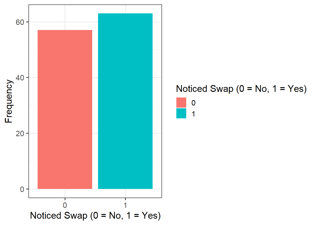
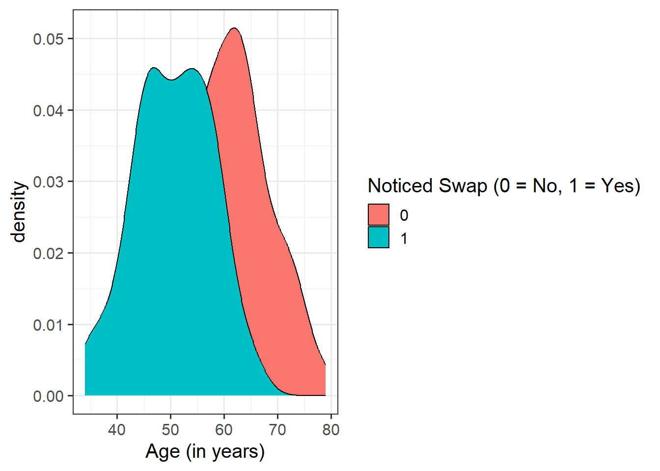
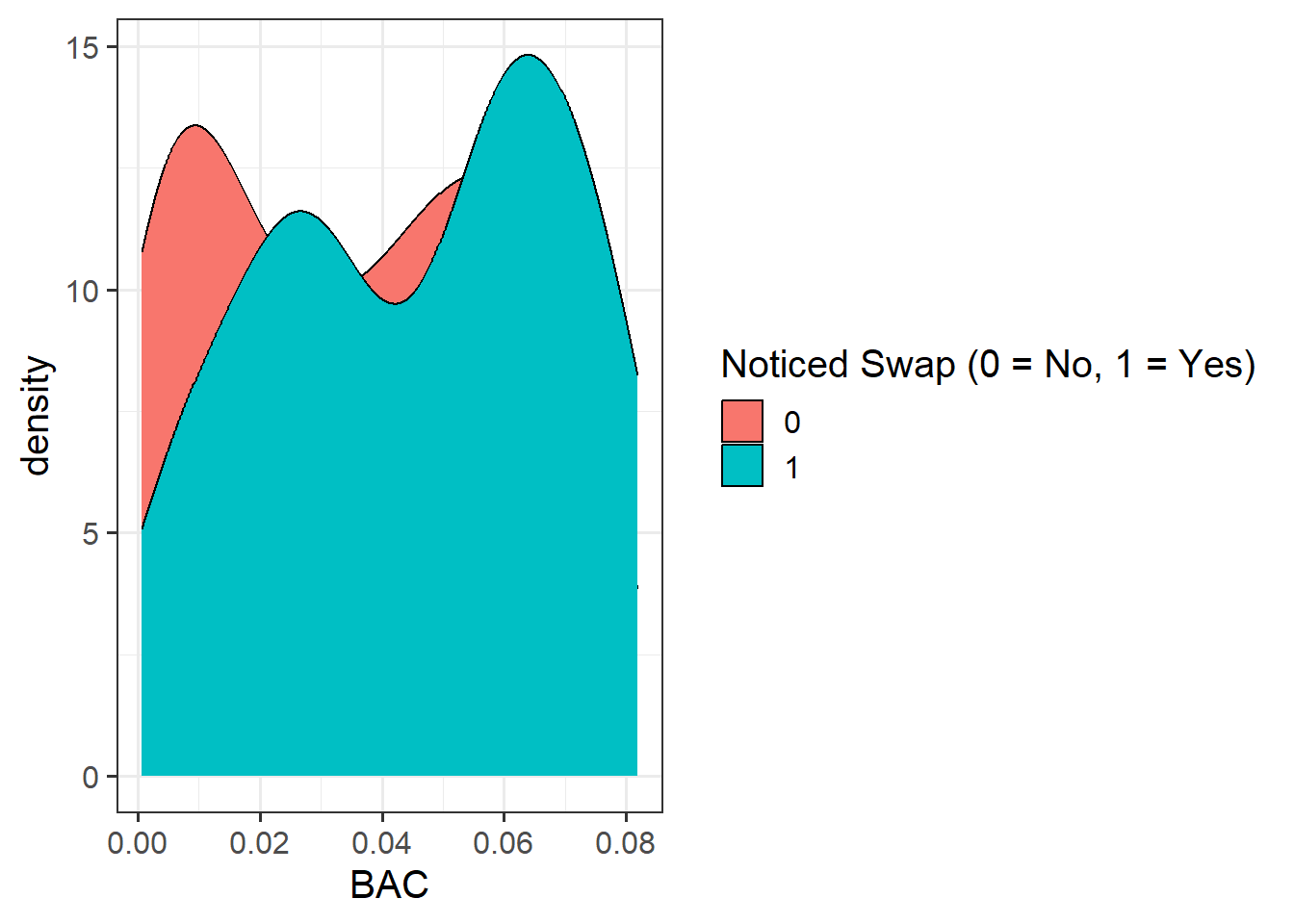
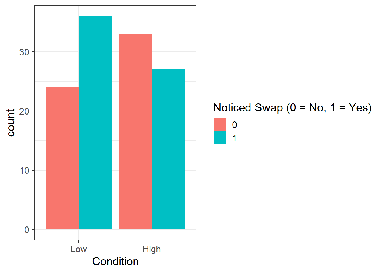
Provide a table of descriptive statistics and visualise your data.

Remember to interpret your plot in the context of the study.

Hint

1. For your table of descriptive statistics, both the group_by() and summarise() functions will come in handy here
2. For your visualisations, you will need to specify as_factor() when plotting the notice variable since this is numeric, but we want it to be treated as a factor only for plotting purposes
3. Make sure to comment on your observations

Solution

Let’s first produce a descriptive statistics table:

door_stats <- drunkdoor %>% 
    group_by(notice, condition) %>%
    summarise(
        Avg_Age = mean(age), 
        SD_Age = sd(age),
        SE_Age = sd(age) / sqrt(n()),
        Min_Age = min(age),
        Max_Age = max(age),        
        Avg_BAC = mean(bac), 
        SD_BAC = sd(bac),
        SE_BAC = sd(bac) / sqrt(n()),
        Min_BAC = min(bac),
        Max_BAC = max(bac)) %>%
    kable(caption = "Descriptive Statistics", digits = 2) %>%
    kable_styling()

door_stats

Table 1: Descriptive Statistics

notice	condition	Avg_Age	SD_Age	SE_Age	Min_Age	Max_Age	Avg_BAC	SD_BAC	SE_BAC	Min_BAC	Max_BAC
0	Low	61.62	8.09	1.65	41	74	0.03	0.02	0	0.00	0.07
0	High	60.21	7.96	1.39	46	79	0.04	0.02	0	0.00	0.08
1	Low	52.42	6.78	1.13	41	65	0.04	0.03	0	0.00	0.08
1	High	47.93	7.05	1.36	34	59	0.05	0.02	0	0.01	0.08

We can explore each of the IVs associations with our DV individually.

Notice

door_plt1 <- ggplot(data = drunkdoor, aes(x=as_factor(notice), fill=as_factor(notice))) +
  geom_bar() +
  labs(x = "Noticed Swap (0 = No, 1 = Yes)", fill = "Noticed Swap (0 = No, 1 = Yes)", y = "Frequency")
door_plt1

Figure 1: Counts of Notice

Notice & Age

door_plt2 <- ggplot(data = drunkdoor, aes(x=age, fill=as_factor(notice))) +
  geom_density() +
  labs(x = "Age (in years)", fill = "Noticed Swap (0 = No, 1 = Yes)")
door_plt2 

Figure 2: Association between Notice and Age

Notice & BAC

door_plt3 <- ggplot(data = drunkdoor, aes(x=bac, fill=as_factor(notice))) +
  geom_density() +
  labs(x = "BAC", fill = "Noticed Swap (0 = No, 1 = Yes)")
door_plt3

Figure 3: Association between Notice and BAC

Notice & Task

door_plt4 <- ggplot(data = drunkdoor, aes(x=condition, fill=as_factor(notice))) +
  geom_bar(position = "dodge") +
  labs(fill = "Noticed Swap (0 = No, 1 = Yes)", x = "Condition")
door_plt4

Figure 4: Association between Notice and Perceptual Load Condition

From Figure 1, we can see that there are slightly more individuals that noticed the mid-conversation swap than those who did not.

From Figure 2, we can see that there appear to be more older adults who did not notice the mid-conversation swap.

From Figure 3, we can see that higher BAC appears to be positively associated with noticing a mid-conversation swap.

From Figure 4, in the Low perceptual load condition, more participants noticed the swap than did not, whilst the opposite pattern emerged in the High perceptual group.

Question 3

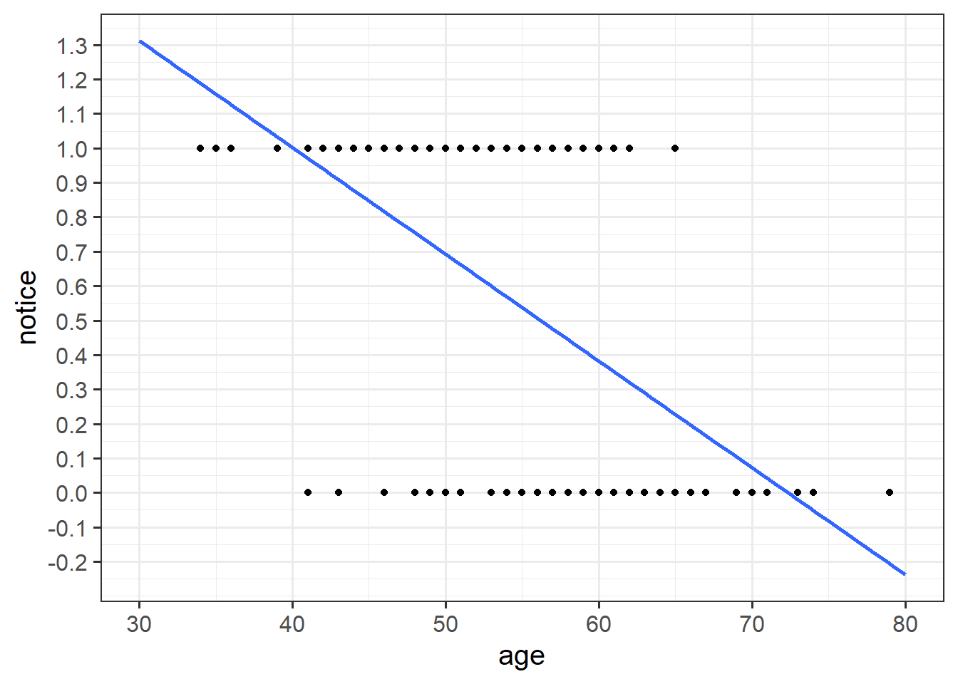
For the moment, lets just consider the association between notice and age. Visually following the line from the plot produced below, what do you think the predicted model value would be for someone who is aged 30? What does this value mean?

Solution

Hopefully you can see that the model predicted value for someone aged 30 is approximately 1.30.

What does 1.30 really mean here? A 30 year old participant will notice 1.30 experimenter-swaps? They have a 130% probability of noticing the swap? That is maybe closer, but we can’t have such a probability - probability is between 0 and 1.

Question 4

Consider the scales that the variables are currently on, with a particular focus on BAC, age, and condition.

• Do you want BAC on the current scale, or could you transform it somehow? Consider that instead of the coefficient representing the difference when moving from 0% to 1% BAC (1% blood alcohol is fatal!), we might want to have the difference associated with 0% to 0.01% BAC (i.e, a we want to talk about effects in terms of changing 1/100th of a percentage of BAC)
• Do you want age to be centred at 0 years (as it currently is), or could you re-centre to make it more meaningful?
• You have hopefully already made condition a factor, but have you considered the reference level? It would likely make most sense for this to be set as “Low”.

Solution

It may be more useful to have blood alcohol (BAC) in terms of 100ths of percentages, rather than percentages, for the reasons noted above.

It would also be more useful for interpretation to have age centered on the mean (note that this won’t change anything other than the intercept in our model).

drunkdoor <- drunkdoor %>% 
  mutate(
    bac100 = bac*100,
    age_mc = age - mean(age)
  )

Now check the condition variable:

#set 'low' as reference group
drunkdoor$condition <- fct_relevel(drunkdoor$condition, "Low")

Question 5

Fit your model using glm(), and assign it as an object with the name “changeblind_mdl”.

Solution

changeblind_mdl <- glm(notice ~ age_mc + bac100 + condition, data = drunkdoor, family = "binomial")
summary(changeblind_mdl)

Call:
glm(formula = notice ~ age_mc + bac100 + condition, family = "binomial", 
    data = drunkdoor)

Deviance Residuals: 
    Min       1Q   Median       3Q      Max  
-3.0505  -0.6747   0.2138   0.6118   2.2543  

Coefficients:
              Estimate Std. Error z value Pr(>|z|)    
(Intercept)   -0.51577    0.53536  -0.963  0.33534    
age_mc        -0.22584    0.04214  -5.359 8.35e-08 ***
bac100         0.35002    0.11128   3.145  0.00166 ** 
conditionHigh -1.59215    0.54008  -2.948  0.00320 ** 
---
Signif. codes:  0 '***' 0.001 '**' 0.01 '*' 0.05 '.' 0.1 ' ' 1

(Dispersion parameter for binomial family taken to be 1)

    Null deviance: 166.06  on 119  degrees of freedom
Residual deviance: 100.99  on 116  degrees of freedom
AIC: 108.99

Number of Fisher Scoring iterations: 5

Question 6

Conduct a model comparison of your model above against the null model. Report the results of the model comparison in APA format.

Hint

Consider whether or not your models are nested. The flowchart in Question 10 of the Semester 2 Week 1 lab may be helpful to revisit.

Solution

#fit null model
changeblind_mdl_null <- glm(notice ~ 1, data = drunkdoor, family = "binomial")

#run model comparison
anova(changeblind_mdl_null, changeblind_mdl, test= "Chisq")

Analysis of Deviance Table

Model 1: notice ~ 1
Model 2: notice ~ age_mc + bac100 + condition
  Resid. Df Resid. Dev Df Deviance  Pr(>Chi)    
1       119     166.06                          
2       116     100.99  3   65.065 4.857e-14 ***
---
Signif. codes:  0 '***' 0.001 '**' 0.01 '*' 0.05 '.' 0.1 ' ' 1

At the 5% significance level, the addition of information about the participants’ age, BAC, and perceptual load resulted in a significant decrease in model deviance \(\chi^2(3) = 65.07, p < .001\).

Hence, we have strong evidence that the participants’ age, BAC, and perceptual load condition are helpful predictors of whether or not they were likely to notice a mid-conversation swap.

Question 7

Interpret your coefficients in the context of the study. When doing so, it may be useful to translate the log-odds back into odds.

Hint

The opposite of the natural logarithm is the exponential, and in R these functions are log() and exp().

Recall that we can obtain our parameter estimates using various functions such as summary(),coef(), coefficients(), etc. Thus, we want to exponentiate the coefficients from our model in order to translate them back from log-odds.

Solution

exp(coefficients(changeblind_mdl))

  (Intercept)        age_mc        bac100 conditionHigh 
    0.5970388     0.7978495     1.4190910     0.2034874 

• \(\beta_0\) = (Intercept) = 0.6
  • The odds of noticing a mid-conversation person-switch for a sober person of average age, with Low perceptual load was 0.60.
• \(\beta_1\) = age_mc = 0.8
  • For every year older someone was, the odds of noticing a mid-conversation sqap reduced by a factor of 0.80, after accounting for differences in blood alcohol levels and perceptual load.
• \(\beta_2\) = bac100 = 1.42
  • For every 1/100th of a percentage increase in BAC, the odds of noticing a mid-conversation person switch increased by a factor of 1.42, after accounting for differences in age and perceptual load.
• \(\beta_3\) conditionHigh = 0.2
  • The odds of noticing the swap were significantly different depending upon the perceptual load. For those in the High perceptual condition, the odds of noticing a change decreased by 0.20, after accounting for differences in age and BAC.

Question 8

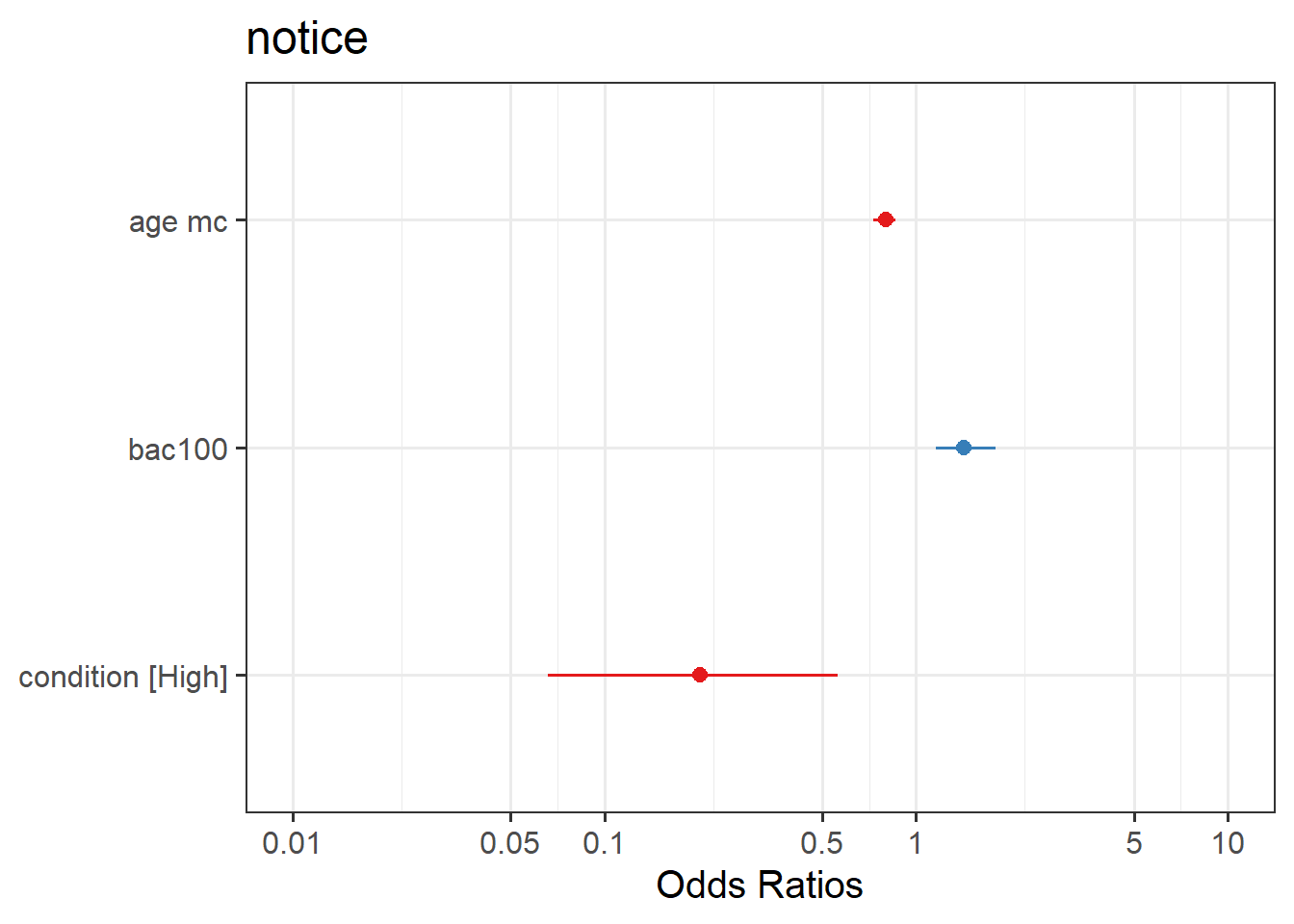
Plot the predicted model estimates.

Hint

Here you will need to use plot_model() from the sjPlot package like you did back in Semester 1. To get your estimates, you will need to specify type = "est".

Solution

plot_model() with type = "est" gives a nice way of visualising the model odds ratios and confidence intervals:

plot_model(changeblind_mdl,
           type = "est")

Figure 5: Model Estimates

Question 9

Provide key model results in a formatted table.

Hint

Use tab_model() from the sjPlot package.

Remember that you can rename your DV and IV labels by specifying dv.labels and pred.labels.

Solution

#create table for results
tab_model(changeblind_mdl,
          dv.labels = "Notice",
          pred.labels = c("age_mc" = "Age (in years)",
                          "bac100" = "Blood Alcohol Level (BAC)",
                          "conditionHigh" = "Condition - High"),
          title = "Regression table for Notice Model")

Table 2: Regression table for Notice model

	Notice
Predictors	Odds Ratios	CI	p
(Intercept)	0.60	0.20 – 1.69	0.335
Age (in years)	0.80	0.73 – 0.86	<0.001
Blood Alcohol Level (BAC)	1.42	1.15 – 1.79	0.002
Condition - High	0.20	0.07 – 0.56	0.003
Observations	120
R2 Tjur	0.475

Question 10

Interpret your results in the context of the research question and report your model in full.

Solution

Make sure to write your results up following APA guidelines:

Whether or not participants noticed the swap mid-conversation (binary 0 vs 1) was modelled using logistic regression, with blood alcohol content (BAC; measured in 100th of percentages blood content), perceptual load condition (low load vs high load, with low as the reference level), and age (in years). See Table 2 for full model results, and Figure 5 for a visualisation of the model estimates and confidence intervals.

Age was found to be associated with susceptibility to change-blindness, as indicated by decreased odds of noting the mid-conversation swap (\(OR = 0.8,\,\, 95\%\, CI\, [0.73, 0.86]\)), after accounting for differences in blood alcohol levels and perceptual load.

In contrary to what might have been expected, change-blindness appeared to decrease with higher alcohol intoxication, with the odds of noticing the swap increasing 1.42 times (\(95\%\, CI\,[1.15, 1.79]\)) for every 1/100th of a percentage increase in blood alcohol content, holding age and perceptual load constant.

After accounting for age and blood alcohol levels, the odds of noticing the swap were significantly different depending upon the perceptual load. For those with a high perceptual load, the odds of noticing a swap decreased by a factor of 0.2 (\(95\%\, CI\,[0.07, 0.56]\)).

In summary, older age increased the susceptibility to change blindness, high perceptual load was found to decrease the chances of people being blind to change, and increased levels of alcohol intoxication appeared to be associated with a greater chance of noticing change.