More Logistic Regression

Learning Objectives

At the end of this lab, you will:

1. Understand when to use a logistic model
2. Understand how to fit and interpret a logistic model
3. Understand how to evaluate model fit

What You Need

1. Be up to date with lectures
2. Have completed previous lab exercises from Week 6

Required R Packages

Remember to load all packages within a code chunk at the start of your RMarkdown file using library(). If you do not have a package and need to install, do so within the console using install.packages(" "). For further guidance on installing/updating packages, see Section C here.

For this lab, you will need to load the following package(s):

• tidyverse
• patchwork
• kableExtra
• psych
• sjPlot

Lab Data

You can download the data required for this lab here or read it in via this link https://uoepsy.github.io/data/QuitAttempts.csv.

Study Overview

Research Question

Is attempting to quit tobacco products associated with an individuals intentions?

Smoking Codebook

Description

Kalkhoran et al. (2015)¹ investigated predictors of dual use of cigarettes and smokeless tobacco products. Although their original sample size was large (\(n\) = 1324), they were interested in running separate logistic regression analyses within subgroups. Most of the sample used only cigarettes. One of the smaller subgroups contained subjects who used both cigarettes and smokeless tobacco products (\(n\)=61). For this problem, we focus on this smaller subgroup of dual cigarette and smokeless tobacco users.

Data Dictionary

variable	description
S	Subject
Q	Quit Attempt, Wheter the subject made an attempt to quit using tobacco products (0 = no attempt to quit; 1 = attempted to quit).
I	Intention to Quit, with four levels: 1 = Never intend to quit; 2 = May intend to quit but not in the next 6 months; 3 = Intend to quit in the next 6 months; 4 = Intend to quit in the next 30 days

Preview

The first six rows of the data are:

S	Q	I
1	0	1
2	1	3
3	1	2
4	0	1
5	1	2
6	1	2

Setup

Setup

1. Create a new RMarkdown file
2. Load the required package(s)
3. Read in the QuitAttempts dataset into R, assigning it to an object named smoke

Solution

#load packages
library(tidyverse)
library(psych)
library(kableExtra)
library(patchwork)
library(sjPlot)

#read in data
smoke <- read_csv("https://uoepsy.github.io/data/QuitAttempts.csv")

Question 1

Examine the dataset, and perform any necessary and appropriate data management steps.

Solution

#look at structure of data:
str(smoke)

spc_tbl_ [62 × 3] (S3: spec_tbl_df/tbl_df/tbl/data.frame)
 $ S: num [1:62] 1 2 3 4 5 6 7 8 9 10 ...
 $ Q: num [1:62] 0 1 1 0 1 1 1 0 1 0 ...
 $ I: num [1:62] 1 3 2 1 2 2 3 3 3 2 ...
 - attr(*, "spec")=
  .. cols(
  ..   S = col_double(),
  ..   Q = col_double(),
  ..   I = col_double()
  .. )
 - attr(*, "problems")=<externalptr> 

#check for NAs - there are none - all FALSE:
table(is.na(smoke))

FALSE 
  186 

#re-name variables to improve clarity:
smoke <- smoke %>%
    rename(PID = S,
           Quit_Attempt = Q,
           Intention = I)

#re-assign categorical IVs as factors, and give more appropriate labels to each level:
smoke$Intention <- factor(smoke$Intention,
                              levels = c(1,2,3,4),
                              labels = c("Never", "Maybe (not in next 6 months)", "Yes (within next 6 months)", "Yes (within next 30 days)"))

Question 2

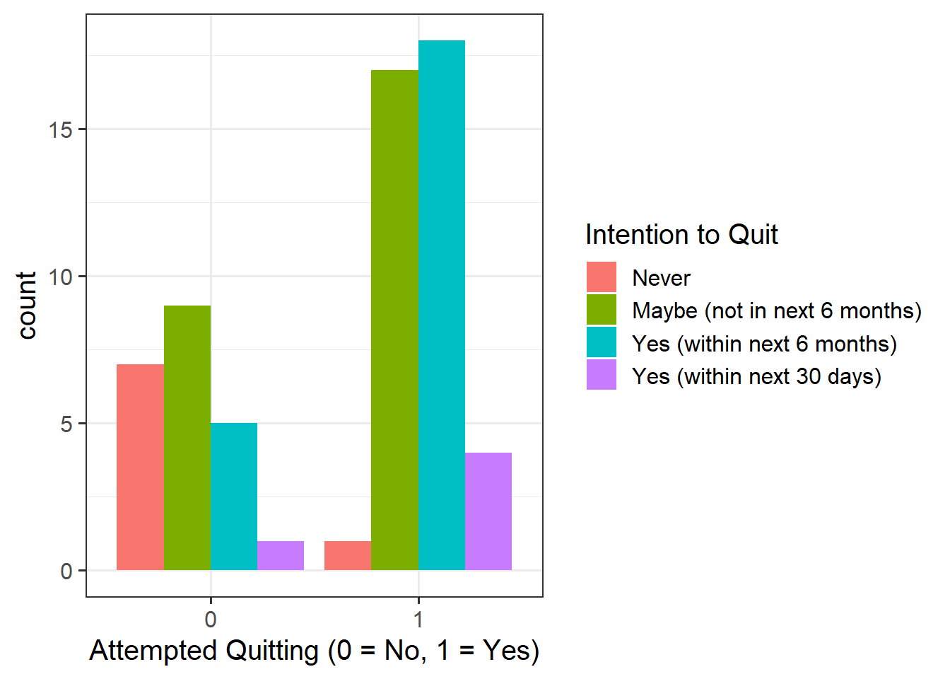
Provide a table of descriptive statistics and visualise your data.

Remember to interpret your plot in the context of the study.

Hint

1. For your table of descriptive statistics, since we have two categorical variables, the select() and table() functions will come in handy here.
2. Recall that when visualising a continuous outcome across several groups, geom_boxplot() may be most appropriate to use.
3. For your visualisations, you will need to specify as_factor() when plotting the Quit_Attempt variable since this is numeric, but we want it to be treated as a factor only for plotting purposes
4. Make sure to comment on any observed differences among the sample means of the four treatment conditions.

Solution

Let’s first produce a descriptive statistics table:

smoke_stats <- smoke %>%
    select(Intention, Quit_Attempt) %>%
    table() %>%
    kable(caption = "Descriptive Statistics") %>%
    kable_styling()

smoke_stats

Table 1: Descriptive Statistics

	0	1
Never	7	1
Maybe (not in next 6 months)	9	17
Yes (within next 6 months)	5	18
Yes (within next 30 days)	1	4

Or alternatively we could view as proportions:

smoke_prop <- smoke %>%
  group_by(Intention, Quit_Attempt) %>%
  summarise(
    n = n()) %>%
  mutate(
    Prop = round(n/sum(n),2)
  ) %>%
    kable(caption = "Proportions") %>%
    kable_styling()

smoke_prop 

Table 2: Proportions

Intention	Quit_Attempt	n	Prop
Never	0	7	0.88
Never	1	1	0.12
Maybe (not in next 6 months)	0	9	0.35
Maybe (not in next 6 months)	1	17	0.65
Yes (within next 6 months)	0	5	0.22
Yes (within next 6 months)	1	18	0.78
Yes (within next 30 days)	0	1	0.20
Yes (within next 30 days)	1	4	0.80

We can explore the association between the two categorical variables as follows:

smoke_plt1 <- ggplot(data = smoke, aes(x=as_factor(Quit_Attempt), fill=Intention)) +
  geom_bar(position = "dodge") +
  labs(fill = 'Intention to Quit', x = "Attempted Quitting (0 = No, 1 = Yes)")
smoke_plt1

Figure 1: Association between Intention and Quitting Attempt

Based on the proportions presented in Table 2, we can see for those who had some intention to quit (i.e., maybe - not in next 6 months, yes - within next 6 months, or yes - within 30 days), there was a larger proportion of individuals who attempted to quit using tobacco products.

From Figure 1, we can see that for those who made an attempt to quit using tobacco products, the majority intended to quit - either in the immediate or distant future. For those who made no attempt to quit using tobacco products, the majority either had no intention of quitting or did not plan to quit in the near future.

Question 3

Fit your model using glm(), and assign it as an object with the name “smoke_mdl1”.

Solution

smoke_mdl1 <- glm(Quit_Attempt ~ Intention, data = smoke, family = "binomial")
summary(smoke_mdl1)

Call:
glm(formula = Quit_Attempt ~ Intention, family = "binomial", 
    data = smoke)

Deviance Residuals: 
    Min       1Q   Median       3Q      Max  
-1.7941  -0.5168   0.7002   0.9218   2.0393  

Coefficients:
                                      Estimate Std. Error z value Pr(>|z|)   
(Intercept)                             -1.946      1.069  -1.820  0.06872 . 
IntentionMaybe (not in next 6 months)    2.582      1.146   2.253  0.02423 * 
IntentionYes (within next 6 months)      3.227      1.183   2.729  0.00636 **
IntentionYes (within next 30 days)       3.332      1.547   2.154  0.03123 * 
---
Signif. codes:  0 '***' 0.001 '**' 0.01 '*' 0.05 '.' 0.1 ' ' 1

(Dispersion parameter for binomial family taken to be 1)

    Null deviance: 80.648  on 61  degrees of freedom
Residual deviance: 68.659  on 58  degrees of freedom
AIC: 76.659

Number of Fisher Scoring iterations: 4

Question 4

Interpret your coefficients in the context of the study. When doing so, it may be useful to translate the log-odds back into odds.

Hint

The opposite of the natural logarithm is the exponential (see here for more details if you are interested), and in R these functions are log() and exp().

Recall that we can obtain our parameter estimates using various functions such as summary(),coef(), coefficients(), etc. Thus, we want to exponentiate the coefficients from our model in order to translate them back from log-odds.

Solution

exp(coefficients(smoke_mdl1))

                          (Intercept) IntentionMaybe (not in next 6 months) 
                            0.1428571                            13.2222222 
  IntentionYes (within next 6 months)    IntentionYes (within next 30 days) 
                           25.2000000                            28.0000000 

• \(\beta_0\) = (Intercept) = 0.14
  • For a participant who reported that they “never intend to quit”, the probability that they did attempt quitting was 0.14 times the probability that they did not.
• \(\beta_1\) = Intention Maybe (not in next 6 months) = 13.22
  • Relative to those who “never intend to quit”, reporting an “intention to quit but not in the next 6 months” meant that an individuals odds of attempting to quit increased by a factor of 13.2.
• \(\beta_2\) = Intention Yes (within next 6 months) = 25.2
  • Relative to those who “never intend to quit”, reporting an “intention to quit in the next 6 months” increased the odds of attempting to quit by a factor of 25.2.
• \(\beta_3\) Intention Yes (within next 30 days) = 28
  • Relative to those who “never intend to quit”, reporting an “intention to quit in the next 30 days” was associated with an increase in the odds of attempting to quit by a factor of 28.

Question 5

Examine the below plot to determine if the deviance residuals raise concerns about outliers:

plot(rstandard(smoke_mdl1, type = 'deviance'), ylab = 'Standardised Deviance Residuals')

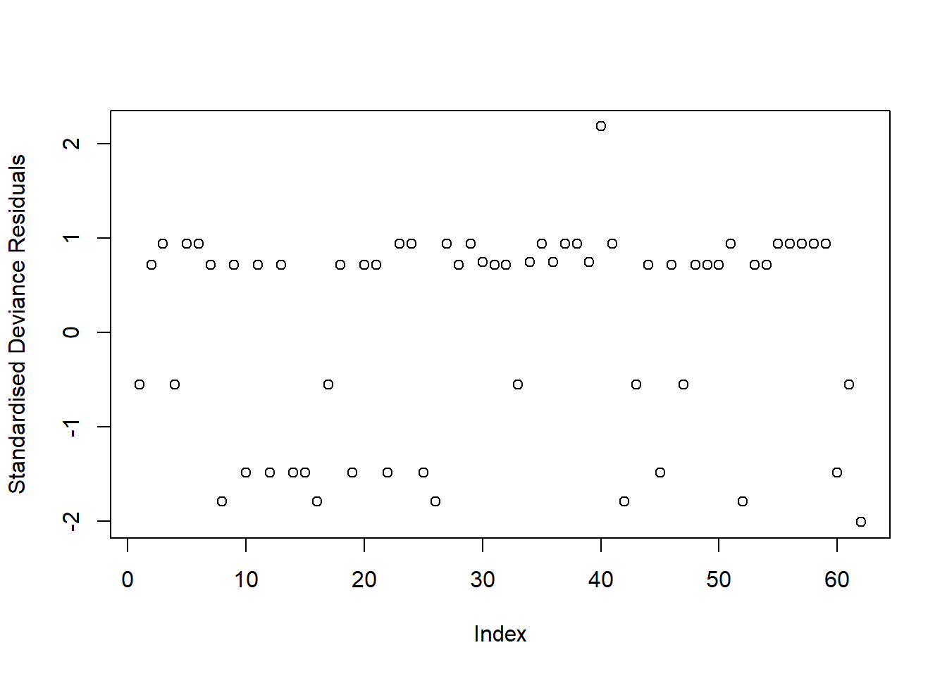
Based on this plot, are there any residuals of concern? Are there any additional plots you could check to determine if there are influential observations?

Hint

Deviance Residuals

Because logistic regression models don’t have the same expected error distribution (we don’t expect residuals to be normally distributed around the mean, with constant variance), checking the assumptions of logistic regression is a little different.

Typically, we look at the “deviance residuals”. But we don’t examine plots for patterns, we simply examine them for potentially outlying observations. If we use a standardised residual, it makes it easier to explore extreme values as we expect most residuals to be within -2, 2 or -3, 3 (depending on how strict we feel).

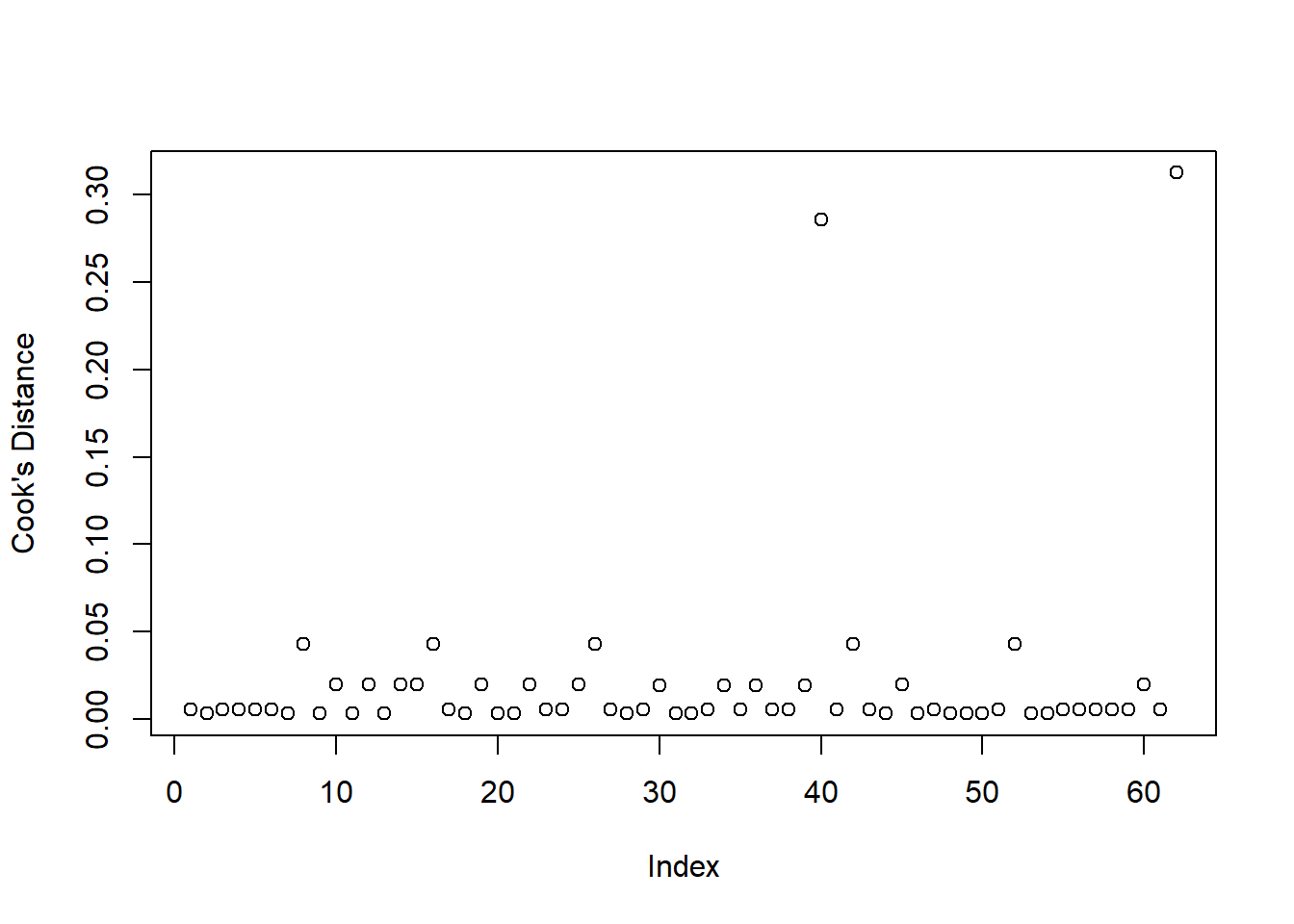
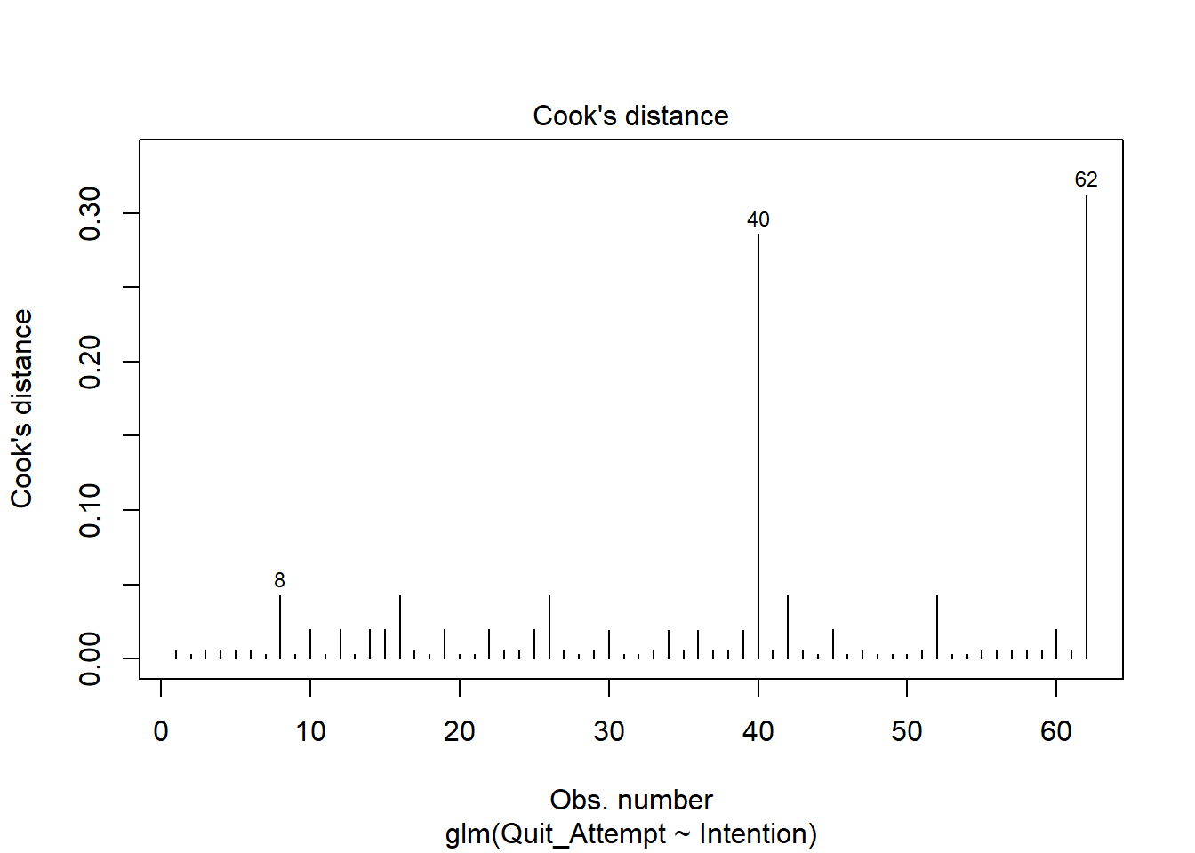
Cook’s Distance

To check for influential observations, we can use cooks.distance(), and plot this using plot(). Alternatively, you can specify which = 4 when plotting your fitted model. In logistic regression, we can use the arbitrary cut-offs of 0.5 (moderately influential) or 1 (highly influential) to describe influential points.

Solution

In the plot above, there appears to be 1 residual with a value >|2|, but none with a value >|3|. We will keep this in mind and check if they are also an influential point by plotting Cook’s Distance:

#cooks d - option 1 (only need to use one of these two options)
plot(cooks.distance(smoke_mdl1), ylab = "Cook's Distance")

#cooks d - option 2 (only need to use one of these two options)
plot(smoke_mdl1, which = 4)

There doesn’t appear to be any influential observations based on our Cook’s distance plot, since all values < .50.

Question 6

Perform a Deviance goodness-of-fit test to compare your fitted model to the null.

\[ \begin{aligned} M_0 &: \qquad \log \left( \frac{p}{1 - p}\right) = \beta_0 \\ M_1 &: \qquad \log \left( \frac{p}{1 - p}\right) = \beta_0 + \beta_1 Intention2 + \beta_2 Intention3 + \beta_3 Intention4 \end{aligned} \]

Report which model you think best fits the data.

Hint

Consider whether or not your models are nested. The flowchart in Question 10 of the Semester 2 Week 1 lab may be helpful to revisit.

Solution

First, let’s fit the null model:

smoke_mdl0 <- glm(Quit_Attempt ~ 1, data = smoke, family = "binomial")
summary(smoke_mdl0)

Call:
glm(formula = Quit_Attempt ~ 1, family = "binomial", data = smoke)

Deviance Residuals: 
    Min       1Q   Median       3Q      Max  
-1.4395  -1.4395   0.9362   0.9362   0.9362  

Coefficients:
            Estimate Std. Error z value Pr(>|z|)  
(Intercept)   0.5978     0.2654   2.252   0.0243 *
---
Signif. codes:  0 '***' 0.001 '**' 0.01 '*' 0.05 '.' 0.1 ' ' 1

(Dispersion parameter for binomial family taken to be 1)

    Null deviance: 80.648  on 61  degrees of freedom
Residual deviance: 80.648  on 61  degrees of freedom
AIC: 82.648

Number of Fisher Scoring iterations: 4

Since our models are nested, we can compare using the likelihood ratio test:

anova(smoke_mdl0, smoke_mdl1, test = 'Chisq')

Analysis of Deviance Table

Model 1: Quit_Attempt ~ 1
Model 2: Quit_Attempt ~ Intention
  Resid. Df Resid. Dev Df Deviance Pr(>Chi)   
1        61     80.648                        
2        58     68.659  3   11.989  0.00742 **
---
Signif. codes:  0 '***' 0.001 '**' 0.01 '*' 0.05 '.' 0.1 ' ' 1

At the 5% significance level, the addition of information about the participants’ intention to quit resulted in a significant decrease in model deviance \(\chi^2(3) = 11.99, p = .007\).

Hence, we have strong evidence that the model the subjects’ intention to quit is a helpful predictor of whether or not they will attempt quitting in the future.

Question 7

Check the AIC and BIC values for smoke_mdl0 and smoke_mdl1 - which model should we prefer?

Solution

#AIC
AIC(smoke_mdl0, smoke_mdl1)

           df      AIC
smoke_mdl0  1 82.64844
smoke_mdl1  4 76.65904

#BIC
BIC(smoke_mdl0, smoke_mdl1)

           df      BIC
smoke_mdl0  1 84.77557
smoke_mdl1  4 85.16758

We used AIC and BIC model selection to distinguish between two possible models describing the association between attempting to quit and intentions. Our model with with intentions included as a predictor (AIC = 76.66) was better fitting than the null model (AIC = 82.65). However, the BIC values suggested that the model including intentions (BIC = 85.17) was a poorer fit than the null (BIC = 84.77). Based on the weight of evidence from both the Deviance goodness-of-fit test alongside the AIC and BIC values, we would conclude that the model with intentions was better fitting than the null.

Question 8

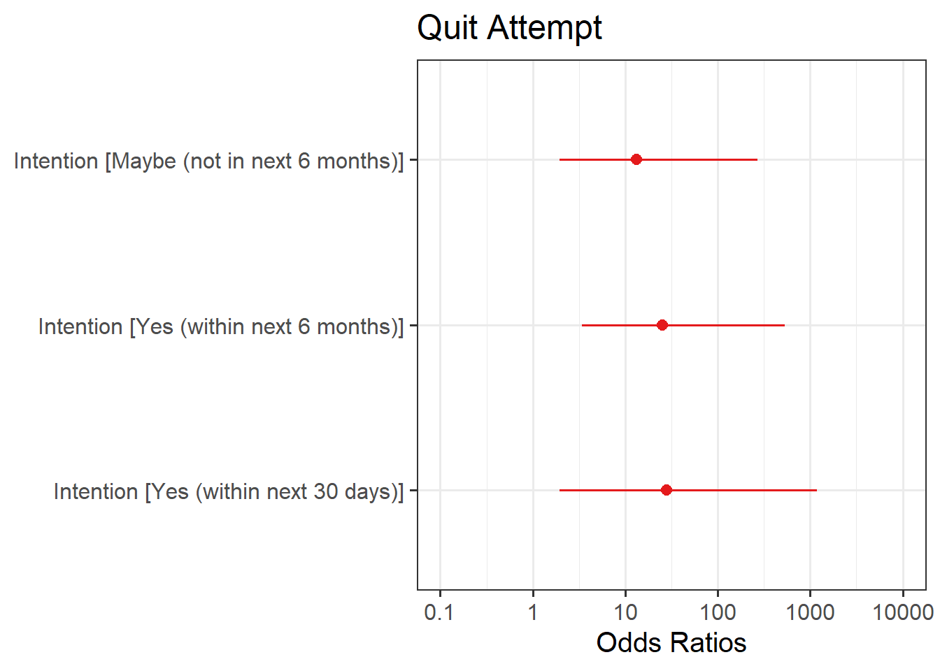
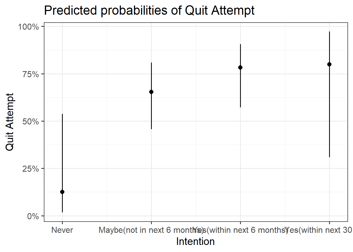
Plot the following:

• predicted model estimates
• predicted probability

Hint

Here you will need to use plot_model() from the sjPlot package like you did back in Semester 1. To get your estimates, you will need to specify type = "est", and for predicted probability, type = "eff".

Solution

plot_model() with type = "est" gives a nice way of visualising the model odds ratios and confidence intervals:

plot_model(smoke_mdl1,
           type = "est")

Figure 2: Model Estimates

plot_model() with type = "eff" allows us to visualise the predicted probability based on our model estimates:

plot_model(smoke_mdl1,
           type = "eff")

$Intention

Figure 3: Predicted Probability

Question 9

Provide key model results in a formatted table.

Hint

Use tab_model() from the sjPlot package.

Remember that you can rename your DV and IV labels by specifying dv.labels and pred.labels.

Solution

#create table for results
tab_model(smoke_mdl1,
          dv.labels = "Attempt to quit using tobacco products",
          pred.labels = c("Maybe (not in next 6 months)" = "Intend to quit but not in the next 6 months",
                          "Yes (within next 6 months)" = "Intend to quit in the next 6 months",
                          "Yes (within next 30 days)" = "Intend to quit in the next 30 days"),
          title = "Regression table for Smoking Model")

Table 3: Regression table for Smoking Model

	Attempt to quit using tobacco products
Predictors	Odds Ratios	CI	p
(Intercept)	0.14	0.01 – 0.80	0.069
IntentionMaybe (not in next 6 months)	13.22	1.93 – 268.17	0.024
IntentionYes (within next 6 months)	25.20	3.42 – 534.12	0.006
IntentionYes (within next 30 days)	28.00	1.95 – 1181.69	0.031
Observations	62
R2 Tjur	0.192

Question 10

Interpret your results in the context of the research question and report your model in full.

Solution

Make sure to write your results up following APA guidelines:

Whether or not participants made an attempt to quit using tobacco products (binary 0 vs 1; 0 no attempt to quit, 1 attempted to quit) was modeled using logistic regression, with intention to quit (‘never intend to quit’, ‘may intend to quit but not in the next 6 months’, ‘intend to quit in the next 6 months’, ‘intend to quit in the next 30 days’, with ‘never intend to quit’ as the reference level) as the only predictor. See Table 3 for full model results, and Figure 2 for a visualisation of the model estimates and confidence intervals.

Having no intention to quit was found to be associated with attempting to quit (\(OR = 0.14,\,\, 95\%\, CI\, [0.01, 0.8]\)), where the probability that they did attempt to quit was 0.14 times the probability that they did not.

Relative to those who never intend to quit, individuals who may intend to quit but not in the next six months had increased odds of attempting to quit (\(OR = 13.22,\,\, 95\%\, CI\, [1.93, 268.17]\)).

In comparison to those with no intention to quit, those who intended to quit in the next six months had their the odds of quitting increased by a factor of 25.2 (\(95\%\, CI\, [3.42, 534.12]\))

Finally, intending to quit in the next 30 days was associated with an increase in the odds of attempting to quit by a factor of 28 (\(95\%\, CI\, [1.95, 1181.69]\)) in comparison to those who never intended to quit.

In summary, the closer in the future someone intended to quit smoking, the higher their odds of attempting to quit using tobacco products (see Figure 3).

Footnotes

1. Kalkhoran, S., Grana, R. A., Neilands, T. B., & Ling, P. M. (2015). Dual use of smokeless tobacco or e-cigarettes with cigarettes and cessation. American Journal of Health Behavior, 39(2), 277–284. https://doi.org/10.5993/AJHB.39.2.14