Model Fit and Standardization

Learning Objectives

At the end of this lab, you will:

1. Understand how to interpret significance tests for \(\beta\) coefficients
2. Understand how to calculate the interpret \(R^2\) and adjusted-\(R^2\) as a measure of model quality.
3. Understand the calculation and interpretation of the \(F\)-test of model utility.
4. Understand how to standardize model coefficients and when this is appropriate to do.

What You Need

1. Be up to date with lectures
2. Have completed previous lab exercises from Week 1, Week 2, and Week 3

Required R Packages

Remember to load all packages within a code chunk at the start of your RMarkdown file using library(). If you do not have a package and need to install, do so within the console using install.packages(" "). For further guidance on installing/updating packages, see Section C here.

For this lab, you will need to load the following package(s):

• tidyverse
• patchwork
• sjPlot

Lab Data

You can download the data required for this lab here or read it in via this link https://uoepsy.github.io/data/wellbeing.csv.

Note: this is the same data as Lab 3.

Study Overview

Research Question

Is there an association between well-being and time spent outdoors after taking into account the association between well-being and social interactions?

Wellbeing data codebook.

Description

Researchers interviewed 32 participants, selected at random from the population of residents of Edinburgh & Lothians. They used the Warwick-Edinburgh Mental Wellbeing Scale (WEMWBS), a self-report measure of mental health and well-being. The scale is scored by summing responses to each item, with items answered on a 1 to 5 Likert scale. The minimum scale score is 14 and the maximum is 70.

The researchers also asked participants to estimate the average number of hours they spend outdoors each week, the average number of social interactions they have each week (whether on-line or in-person), and whether they believe that they stick to a routine throughout the week (Yes/No).

The data in wellbeing.csv contain five attributes collected from a random sample of \(n=32\) hypothetical residents over Edinburgh & Lothians, and include:

• wellbeing: Warwick-Edinburgh Mental Wellbeing Scale (WEMWBS), a self-report measure of mental health and well-being. The scale is scored by summing responses to each item, with items answered on a 1 to 5 Likert scale. The minimum scale score is 14 and the maximum is 70.
  
• outdoor_time: Self report estimated number of hours per week spent outdoors
  
• social_int: Self report estimated number of social interactions per week (both online and in-person)
• routine: Binary Yes/No response to the question “Do you follow a daily routine throughout the week?”
• location: Location of primary residence (City, Suburb, Rural)

Preview

The first six rows of the data are:

wellbeing	outdoor_time	social_int	location	routine
30	7	8	Suburb	Routine
21	9	8	City	No Routine
38	14	10	Suburb	Routine
27	16	10	City	No Routine
20	1	10	Rural	No Routine
37	11	12	Suburb	No Routine

Setup

Setup

1. Create a new RMarkdown file
2. Load the required package(s)
3. Read the wellbeing dataset into R, assigning it to an object named mwdata

Solution

#Loading the required package(s)
library(tidyverse)
library(patchwork)
library(sjPlot)

# Reading in data and storing to an object named 'mwdata'
mwdata <- read_csv("https://uoepsy.github.io/data/wellbeing.csv")

Exercises

Question 1

Specify and fit a linear model to investigate how wellbeing (WEMWBS scores) are associated with time spent outdoors after controlling for the number of social interactions.

Next, check the summary() output from the model.

Solution

The model is: \[ \widehat{Wellbeing} = \hat \beta_0 + \hat \beta_1 \cdot Social Interactions + \hat \beta_2 \cdot Outdoor Time \] In R:

#fit model
mdl1 <- lm(wellbeing ~ social_int + outdoor_time, data = mwdata)

#look at summary output from model
summary(mdl1)

Call:
lm(formula = wellbeing ~ social_int + outdoor_time, data = mwdata)

Residuals:
   Min     1Q Median     3Q    Max 
-9.742 -4.915 -1.255  5.628 10.936 

Coefficients:
             Estimate Std. Error t value Pr(>|t|)    
(Intercept)    5.3704     4.3205   1.243   0.2238    
social_int     1.8034     0.2691   6.702 2.37e-07 ***
outdoor_time   0.5924     0.1689   3.506   0.0015 ** 
---
Signif. codes:  0 '***' 0.001 '**' 0.01 '*' 0.05 '.' 0.1 ' ' 1

Residual standard error: 6.148 on 29 degrees of freedom
Multiple R-squared:  0.7404,    Adjusted R-squared:  0.7224 
F-statistic: 41.34 on 2 and 29 DF,  p-value: 3.226e-09

Question 2

Formally state:

• your chosen significance level
• the null and alternative hypotheses

Solution

Effects will be considered statistically significant at \(\alpha=.05\)

\(H_0: \beta_2 = 0\)

There is no association between well-being and time spent outdoors after taking into account the relationship between well-being and social interactions

\(H_1: \beta_2 \neq 0\)

There is an association between well-being and time spent outdoors after taking into account the relationship between well-being and social interactions

Lab Purpose

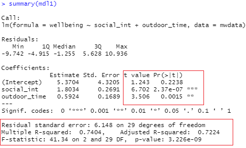
In this lab (Lab 4), you will focus on the statistics contained within the highlighted sections of the summary() output below. You will be both calculating these by hand and deriving via R code before interpreting these values in the context of the research question following APA guidelines.

Question 3

Test the hypothesis that the population slope for outdoor time is zero — that is, that there is no linear association between wellbeing and outdoor time (after controlling for the number of social interactions) in the population.

Hint

Recall the formula for obtaining a test statistic:

A test statistic for the null hypothesis \(H_0: \beta_j = 0\) is \[ t = \frac{\hat \beta_j - 0}{SE(\hat \beta_j)} \] which follows a \(t\)-distribution with \(n-k-1 = n - 2 - 1 = n - 3\) degrees of freedom.

Solution

Manually

We calculate the test statistic for \(\beta_2\) \[ t = \frac{\hat \beta_2 - 0}{SE(\hat \beta_2)} = \frac{0.5924 - 0}{0.1689} = 3.5074 \]

and compare it with the 5% critical value from a \(t\)-distribution with \(n-3\) degrees of freedom, which is:

n <- nrow(mwdata)
tstar <- qt(0.975, df = n - 3)
tstar

[1] 2.04523

#tstar = 2.04523

As \(|t|\) (\(|t|\) = 3.51) is much larger than \(t^*\) (\(t^*\) = 2.05), we can reject then null hypothesis as we have strong evidence against it.

The \(p\)-value, shown below, also confirms this conclusion.

2 * (1 - pt(3.506, n - 3))

[1] 0.001500588

R function

Please note that the same information was already contained in the row corresponding to the variable “outdoor_time” in the output of summary(mdl), which reported the \(t\)-statistic under t value and the \(p\)-value under Pr(>|t|):

summary(mdl1)

Call:
lm(formula = wellbeing ~ social_int + outdoor_time, data = mwdata)

Residuals:
   Min     1Q Median     3Q    Max 
-9.742 -4.915 -1.255  5.628 10.936 

Coefficients:
             Estimate Std. Error t value Pr(>|t|)    
(Intercept)    5.3704     4.3205   1.243   0.2238    
social_int     1.8034     0.2691   6.702 2.37e-07 ***
outdoor_time   0.5924     0.1689   3.506   0.0015 ** 
---
Signif. codes:  0 '***' 0.001 '**' 0.01 '*' 0.05 '.' 0.1 ' ' 1

Residual standard error: 6.148 on 29 degrees of freedom
Multiple R-squared:  0.7404,    Adjusted R-squared:  0.7224 
F-statistic: 41.34 on 2 and 29 DF,  p-value: 3.226e-09

The result is exactly the same (up to rounding errors) as calculating manually.

Before we interpret the results, note that sometimes \(p\)-values will be reported to \(e^X\). For example, look in the Pr(>|t|) column for “social_int”. The value \(2.37e^{-07}\) simply means \(2.37 \times 10^{-7}\). This is a very small value (i.e., 0.000000237), hence we will report it as <.001 following the APA guidelines.

We performed a \(t\)-test against the null hypothesis that outdoor time was not associated with wellbeing scores after controlling for social interactions. A significant association was found between outdoor time (in hours per week) and wellbeing (WEMWBS scores) \(t(29) = 3.51,\ p = 002\), two-sided. Thus, we have evidence to reject the null hypothesis.

Question 4

Obtain 95% confidence intervals for the regression coefficients, and write a sentence about each one.

Hint

Recall the formula for obtaining a confidence interval:

A confidence interval for the population slope is \[ \hat \beta_j \pm t^* \cdot SE(\hat \beta_j) \] where \(t^*\) denotes the critical value chosen from t-distribution with \(n-k-1 = n - 2 - 1 = n - 3\) degrees of freedom for a desired \(\alpha\) level of confidence.

Solution

Manually

For 95% confidence we have \(t^* = 2.05\):

n <- nrow(mwdata)
tstar <- qt(0.975, df = n - 3)
tstar

[1] 2.04523

The confidence intervals are:

tibble(
  b0_LowerCI = round(5.3704 - (qt(0.975, n-3) * 4.3205), 3),
  b0_UpperCI = round(5.3704 + (qt(0.975, n-3)* 4.3205), 3),
  b1_LowerCI = round(1.8034 - (qt(0.975, n-3) * 0.2691), 3),
  b1_UpperCI = round(1.8034 + (qt(0.975, n-3)* 0.2691), 3),
  b2_LowerCI = round(0.5924 - (qt(0.975, n-3) * 0.1689), 3),
  b2_UpperCI = round(0.5924 + (qt(0.975, n-3)* 0.1689), 3)
      )

# A tibble: 1 × 6
  b0_LowerCI b0_UpperCI b1_LowerCI b1_UpperCI b2_LowerCI b2_UpperCI
       <dbl>      <dbl>      <dbl>      <dbl>      <dbl>      <dbl>
1      -3.47       14.2       1.25       2.35      0.247      0.938

R function

We can easily obtain the confidence intervals for the regression coefficients using the command confint():

confint(mdl1, level = 0.95)

                  2.5 %     97.5 %
(Intercept)  -3.4660660 14.2068209
social_int    1.2530813  2.3538164
outdoor_time  0.2468371  0.9378975

The result is exactly the same (up to rounding errors) as calculating manually.

• The average wellbeing score for all those with zero hours of outdoor time and zero social interactions per week was between -3.47 and 14.21.
  
• When holding weekly outdoor time constant, each increase of one social interaction per week was associated with a difference in wellbeing scores between 1.25 and 2.35, on average.
  
• When holding the number of social interactions per week constant, each one hour increase in weekly outdoor time was associated with a difference in wellbeing scores between 0.25 and 0.94, on average.

Question 5

What is the proportion of the total variability in wellbeing scores explained by the model?

Hint

The question asks to compute the value of \(R^2\). Since the model includes 2 predictors, you should report the Adjusted \(R^2\).

Solution

The proportion of the total variability explained is given by R-squared.

The R-squared coefficient is defined as: \[ R^2 = \frac{SS_{Model}}{SS_{Total}} = 1 - \frac{SS_{Residual}}{SS_{Total}} \] The Adjusted R-squared coefficient is defined as:

\[ \hat R^2 = 1 - \frac{(1 - R^2)(n-1)}{n-k-1} \quad \\ \begin{align} & \text{Where:} \\ & n = \text{sample size} \\ & k = \text{number of explanatory variables} \\ \end{align} \] ::: {.panel-tabset}

Manually

In R we can write:

#R squared & adjusted R squared

wellbeing_fitted <- mwdata %>%
  mutate(
    wellbeing_hat = predict(mdl1),
    resid = wellbeing - wellbeing_hat
  )


wellbeing_fitted %>%
  summarise(
    SSModel = sum( (wellbeing_hat - mean(wellbeing))^2 ),
    SSTotal = sum( (wellbeing - mean(wellbeing))^2 )
  ) %>%
  summarise(
    RSquared = SSModel / SSTotal,
    AdjRSquared = 1-((1-(RSquared))*(32-1)/(32-2-1))
  )

# A tibble: 1 × 2
  RSquared AdjRSquared
     <dbl>       <dbl>
1    0.740       0.722

R function

#look in second bottom row - Multiple R Squared and Adjusted R Squared both reported here
summary(mdl1)

Call:
lm(formula = wellbeing ~ social_int + outdoor_time, data = mwdata)

Residuals:
   Min     1Q Median     3Q    Max 
-9.742 -4.915 -1.255  5.628 10.936 

Coefficients:
             Estimate Std. Error t value Pr(>|t|)    
(Intercept)    5.3704     4.3205   1.243   0.2238    
social_int     1.8034     0.2691   6.702 2.37e-07 ***
outdoor_time   0.5924     0.1689   3.506   0.0015 ** 
---
Signif. codes:  0 '***' 0.001 '**' 0.01 '*' 0.05 '.' 0.1 ' ' 1

Residual standard error: 6.148 on 29 degrees of freedom
Multiple R-squared:  0.7404,    Adjusted R-squared:  0.7224 
F-statistic: 41.34 on 2 and 29 DF,  p-value: 3.226e-09

The output of summary() displays the Adjusted \(R\)-squared value in the following line:

Adjusted R-squared:  0.7224 

:::

---

Interpretation

Approximately 72% of the total variability in wellbeing scores is explained by associations with social interactions and outdoor time.

Question 6

Perform a model utility test at the 5% significance level and report your results.

In other words, conduct an \(F\)-test against the null hypothesis that the model is ineffective at predicting wellbeing scores using social interactions and outdoor time by computing the \(F\)-statistic using its definition.

Hint

The F-ratio is used to test the null hypothesis that all regression slopes are zero.
It is called the F-ratio because it is the ratio of the how much of the variation is explained by the model (per paramater) versus how much of the variation is left unexplained in the residuals (per remaining degrees of freedom).

\[ F_{df_{model},df_{residual}} = \frac{MS_{Model}}{MS_{Residual}} = \frac{SS_{Model}/df_{Model}}{SS_{Residual}/df_{Residual}} \\ \quad \\ \begin{align} & \text{Where:} \\ & df_{model} = k \\ & df_{residual} = n-k-1 \\ & n = \text{sample size} \\ & k = \text{number of explanatory variables} \\ \end{align} \]

Solution

Manually

df1 <- 2
df2 <- nrow(mwdata) - 2 - 1
f_star <- qf(0.95, df1, df2)
f_star

[1] 3.327654

model_utility <- wellbeing_fitted %>%
  summarise(
    SSModel = sum((wellbeing_hat - mean(wellbeing))^2 ),
    SSResid = sum( resid^2 ),
    MSModel = SSModel / df1,
    MSResid = SSResid / df2,
    FObs = MSModel / MSResid
  )
model_utility

# A tibble: 1 × 5
  SSModel SSResid MSModel MSResid  FObs
    <dbl>   <dbl>   <dbl>   <dbl> <dbl>
1   3126.   1096.   1563.    37.8  41.3

We can also compute the p-value:

pvalue <- 1 - pf(model_utility$FObs, df1, df2)
pvalue

[1] 3.225548e-09

The value 3.225548e-09 simply means \(3.2 \times 10^{-9}\), so it’s a really small number.

R function

#look in bottom row
summary(mdl1)

Call:
lm(formula = wellbeing ~ social_int + outdoor_time, data = mwdata)

Residuals:
   Min     1Q Median     3Q    Max 
-9.742 -4.915 -1.255  5.628 10.936 

Coefficients:
             Estimate Std. Error t value Pr(>|t|)    
(Intercept)    5.3704     4.3205   1.243   0.2238    
social_int     1.8034     0.2691   6.702 2.37e-07 ***
outdoor_time   0.5924     0.1689   3.506   0.0015 ** 
---
Signif. codes:  0 '***' 0.001 '**' 0.01 '*' 0.05 '.' 0.1 ' ' 1

Residual standard error: 6.148 on 29 degrees of freedom
Multiple R-squared:  0.7404,    Adjusted R-squared:  0.7224 
F-statistic: 41.34 on 2 and 29 DF,  p-value: 3.226e-09

The relevant row is the following:

F-statistic: 41.34 on 2 and 29 DF,  p-value: 3.226e-09

We performed an \(F\)-test of model utility at the 5% significance level, where \(F(2,29) = 41.34, p <.001\).

The large \(F\)-statistic and small \(p\)-value (\(<.001\)) suggested that we have very strong evidence against the null hypothesis that the model is ineffective.

In other words, the data provide strong evidence that the number of social interactions and outdoor time are effective predictors of wellbeing scores.

Question 7

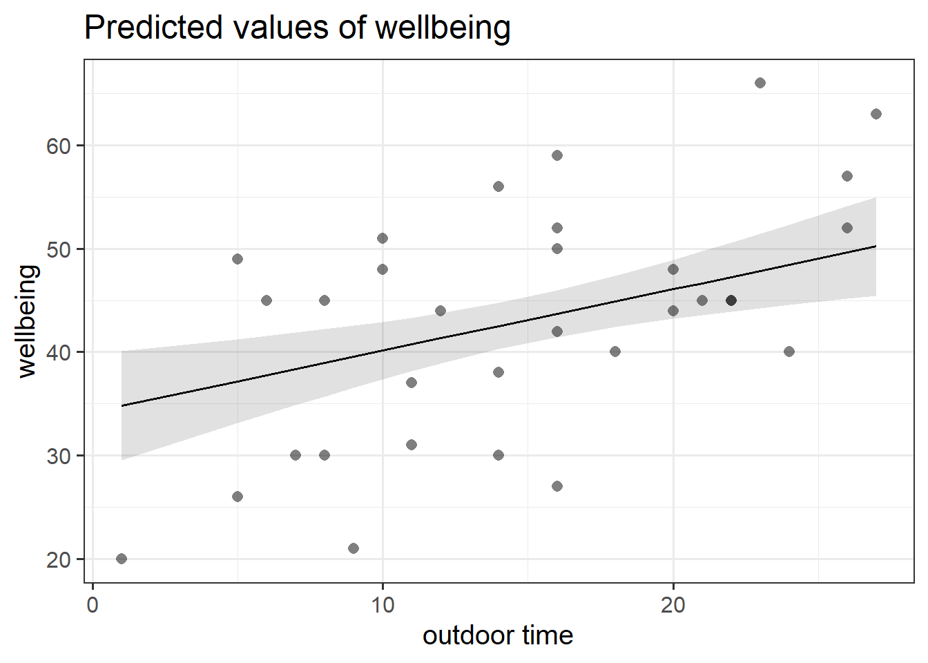
Produce a visualisation of the association between wellbeing and outdoor time, after accounting for social interactions.

Hint

To visualise just one association, you might need to specify the terms argument in plot_model(). Don’t forget you can look up the documentation by typing ?plot_model in the console.

Solution

plot_model(mdl1, type = "eff",
           terms = c("outdoor_time"), 
           show.data = TRUE)

Standardization

Question 8

Fit the regression model using the standardized response and explanatory variables.

Hint

You can either:

1. Add to the “mwdata” dataset three variables called z_wellbeing, z_social_int, and z_outdoor_time representing the standardized welllbeing, social interactions and outdoor time variables, respectively.

Recall the formula for the \(z\)-score: \[ z_x = \frac{x - \bar{x}}{s_x}, \qquad z_y = \frac{y - \bar{y}}{s_y} \]

OR

2. Use the scale() function when specifying your lm() statement.

Solution

Z-Score

z score variables

mwdata <- mwdata %>%
  mutate(
    z_wellbeing = (wellbeing - mean(wellbeing)) / sd(wellbeing),
    z_social_int = (social_int - mean(social_int)) / sd(social_int),
    z_outdoor_time = (outdoor_time - mean(outdoor_time)) / sd(outdoor_time)
  )

Check that they are standardized

mwdata %>%
  summarise(
    M_z_wellbeing = round(mean(z_wellbeing),2), SD_z_wellbeing = sd(z_wellbeing), 
    M_z_social_int = round(mean(z_social_int),2), SD_z_social_int = sd(z_social_int),
    M_z_outdoor_time = round(mean(z_outdoor_time),2), SD_z_outdoor_time = sd(z_outdoor_time)
  )

# A tibble: 1 × 6
  M_z_wellbeing SD_z_wellbeing M_z_social_int SD_z_social_int M_z_outd…¹ SD_z_…²
          <dbl>          <dbl>          <dbl>           <dbl>      <dbl>   <dbl>
1             0              1              0               1          0       1
# … with abbreviated variable names ¹​M_z_outdoor_time, ²​SD_z_outdoor_time

#mean of 0, SD of 1 - all good to go

Run model

#with z scoring
mdl_z <- lm(z_wellbeing ~ z_social_int + z_outdoor_time, data = mwdata)
summary(mdl_z)

Call:
lm(formula = z_wellbeing ~ z_social_int + z_outdoor_time, data = mwdata)

Residuals:
    Min      1Q  Median      3Q     Max 
-0.8347 -0.4212 -0.1075  0.4822  0.9371 

Coefficients:
                Estimate Std. Error t value Pr(>|t|)    
(Intercept)    1.327e-16  9.313e-02   0.000   1.0000    
z_social_int   6.742e-01  1.006e-01   6.702 2.37e-07 ***
z_outdoor_time 3.527e-01  1.006e-01   3.506   0.0015 ** 
---
Signif. codes:  0 '***' 0.001 '**' 0.01 '*' 0.05 '.' 0.1 ' ' 1

Residual standard error: 0.5268 on 29 degrees of freedom
Multiple R-squared:  0.7404,    Adjusted R-squared:  0.7224 
F-statistic: 41.34 on 2 and 29 DF,  p-value: 3.226e-09

round(summary(mdl_z)$coefficients,3)

               Estimate Std. Error t value Pr(>|t|)
(Intercept)       0.000      0.093   0.000    1.000
z_social_int      0.674      0.101   6.702    0.000
z_outdoor_time    0.353      0.101   3.506    0.001

scale function

mdl_s <- lm(scale(wellbeing) ~ scale(social_int) + scale(outdoor_time), data = mwdata)
summary(mdl_s)

Call:
lm(formula = scale(wellbeing) ~ scale(social_int) + scale(outdoor_time), 
    data = mwdata)

Residuals:
    Min      1Q  Median      3Q     Max 
-0.8347 -0.4212 -0.1075  0.4822  0.9371 

Coefficients:
                     Estimate Std. Error t value Pr(>|t|)    
(Intercept)         1.327e-16  9.313e-02   0.000   1.0000    
scale(social_int)   6.742e-01  1.006e-01   6.702 2.37e-07 ***
scale(outdoor_time) 3.527e-01  1.006e-01   3.506   0.0015 ** 
---
Signif. codes:  0 '***' 0.001 '**' 0.01 '*' 0.05 '.' 0.1 ' ' 1

Residual standard error: 0.5268 on 29 degrees of freedom
Multiple R-squared:  0.7404,    Adjusted R-squared:  0.7224 
F-statistic: 41.34 on 2 and 29 DF,  p-value: 3.226e-09

round(summary(mdl_s)$coefficients,3)

                    Estimate Std. Error t value Pr(>|t|)
(Intercept)            0.000      0.093   0.000    1.000
scale(social_int)      0.674      0.101   6.702    0.000
scale(outdoor_time)    0.353      0.101   3.506    0.001

From comparing either the summary() or rounded output, you should see that the estimates are the same under both approaches.

Question 9

Create a table to present your results from the standardized model.

Hint

Use tab_model() from the sjPlot package.

Remember that you can rename your DV and IV labels by specifying dv.labels and pred.labels.

Solution

tab_model(mdl_z,
          dv.labels = "Wellbeing (WEMWBS Scores)",
          pred.labels = c("z_social_int" = "Social Interactions (number per week)",
                          "z_outdoor_time" = "Outdoor Time (hours per week)"),
          title = "Regression table for Wellbeing model. Outcome variable and predictors are Z-scored")

Regression table for Wellbeing model. Outcome variable and predictors are Z-scored

	Wellbeing (WEMWBS Scores)
Predictors	Estimates	CI	p
(Intercept)	0.00	-0.19 – 0.19	1.000
Social Interactions (number per week)	0.67	0.47 – 0.88	<0.001
Outdoor Time (hours per week)	0.35	0.15 – 0.56	0.001
Observations	32
R2 / R2 adjusted	0.740 / 0.722

Question 10

Interpret the standardized variables presented in the above table.

Solution

• For every standard deviation increase in social interactions, wellbeing scores increased on average by 0.67 standard deviations.
• For every standard deviation increase in outdoor time, wellbeing scores increased on average by 0.35 standard deviations.