Interactions II: Num x Num

Learning Objectives

At the end of this lab, you will:

1. Understand the concept of an interaction.
2. Be able to interpret the meaning of a numeric \(\times\) numeric interaction.
3. Understand the principle of marginality and why this impacts modelling choices with interactions.
4. Visualize and probe interactions.

What You Need

1. Be up to date with lectures
2. Have completed previous lab exercises from Week 7

Required R Packages

Remember to load all packages within a code chunk at the start of your RMarkdown file using library(). If you do not have a package and need to install, do so within the console using install.packages(" "). For further guidance on installing/updating packages, see Section C here.

For this lab, you will need to load the following package(s):

• tidyverse
• psych
• sjPlot
• kableExtra
• sandwich
• interactions

Lab Data

You can download the data required for this lab here or read it in via this link https://uoepsy.github.io/data/scs_study.csv.

Study Overview

Research Question

Does the effect of social comparison on symptoms of depression, anxiety and stress vary depending on level of Neuroticism?

Previous research has identified an association between an individual’s perception of their social rank and symptoms of depression, anxiety and stress. We are interested in the individual differences in this association.

To investigate whether the effect of social comparison on symptoms of depression, anxiety and stress varies depending on level of Neuroticism, we will need to fit a multiple regression model with an interaction term. Before we think about fitting our model, it is important that we understand the data available - how many participants? What type (or class) of data will we be working with? What was the measurement scale? How were scales scored? Look at the social comparison study data codebook below.

Social Comparison Study data codebook

Description

Data from 656 participants containing information on scores on each trait of a Big 5 personality measure, their perception of their own social rank, and their scores on a measure of depression.

The data in scs_study.csv contain seven attributes collected from a random sample of \(n=656\) participants:

• zo: Openness (Z-scored), measured on the Big-5 Aspects Scale (BFAS)
• zc: Conscientiousness (Z-scored), measured on the Big-5 Aspects Scale (BFAS)
• ze: Extraversion (Z-scored), measured on the Big-5 Aspects Scale (BFAS)
• za: Agreeableness (Z-scored), measured on the Big-5 Aspects Scale (BFAS)
• zn: Neuroticism (Z-scored), measured on the Big-5 Aspects Scale (BFAS)
• scs: Social Comparison Scale - An 11-item scale that measures an individual’s perception of their social rank, attractiveness and belonging relative to others. The scale is scored as a sum of the 11 items (each measured on a 5-point scale), with higher scores indicating more favourable perceptions of social rank.
• dass: Depression Anxiety and Stress Scale - The DASS-21 includes 21 items, each measured on a 4-point scale. The score is derived from the sum of all 21 items, with higher scores indicating higher a severity of symptoms.

Preview

The first six rows of the data are:

zo	zc	ze	za	zn	scs	dass
0.76	1.58	-0.79	-0.09	1.32	30	56
0.30	-0.27	-0.09	0.09	-0.40	30	48
-0.13	0.66	-0.80	-0.95	0.93	35	48
1.06	-1.02	-0.16	-0.50	-0.02	29	48
1.74	-0.78	-1.55	-2.86	-1.14	41	43
0.22	-0.41	0.78	0.90	-0.25	37	60

Setup

Setup

1. Create a new RMarkdown file
2. Load the required package(s)
3. Read the scs_study dataset into R, assigning it to an object named scs_study

Solution

#Loading the required package(s)
library(tidyverse)
library(psych)
library(sjPlot)
library(kableExtra) 
library(sandwich)
library(interactions)

#Reading in data and storing in object named 'scs_study'
scs_study <- read_csv("https://uoepsy.github.io/data/scs_study.csv")

Exercises

Question 1

Formally state:

• a linear model to investigate whether the effect of social comparison on symptoms of depression, anxiety and stress varies depending on level of Neuroticism
• your chosen significance level
• the null and alternative hypotheses

Solution

\[ {DASS-21 Score} = \beta_0 + \beta_1 \cdot SCS Score + \beta_2 \cdot Neuroticism + \beta_3 \cdot (SCS Score \cdot Neuroticism) \] Effects will be considered statistically significant at \(\alpha=.05\)

Our hypotheses are:

\(H_0: \beta_3 = 0\)

The effect of social comparison on symptoms of depression, anxiety and stress does not vary depending on level of Neuroticism

\(H_1: \beta_3 \neq 0\)

The effect of social comparison on symptoms of depression, anxiety and stress does vary depending on level of Neuroticism.

Question 2

Provide a table of descriptive statistics and visualise your data.

Remember to interpret these plots in the context of the study.

Hint

1. The describe() function is from the psych package; and kable() and kable_styling() (which are used to make a nice table) from kableExtra would be useful to present your descriptive statistics.
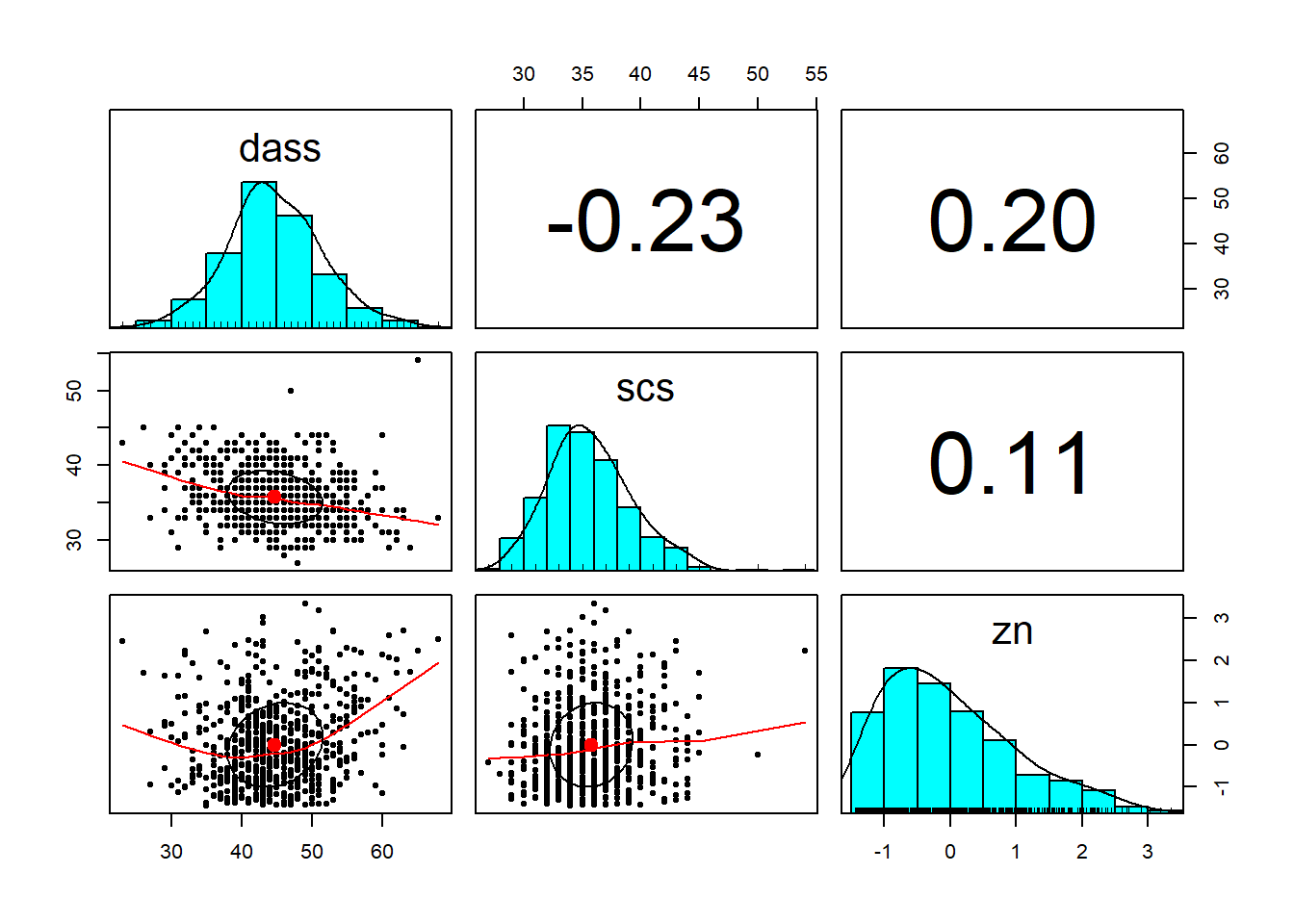
2. The pairs.panels() function from the psych package will plot all variables in a dataset against one another. This will save you the time you would have spent creating individual plots.

Solution

First, lets look at our descriptive statistics and present in a well formatted table:

# note that we are selecting our three variables of interest (dass, scs, zn)
# we are then passing these to the kable() and kable_styling() functions so that we end up with a nice looking table, and specify digits = 2 so that output is rounded to 2 decimal places

describe(scs_study %>% 
             select(dass, scs, zn)) %>% 
             kable(caption = "Descriptive Statistics - DASS-21, SCS, and Neuroticism (Z-Scored)", digits = 2) %>%
             kable_styling()

Table 1: Descriptive Statistics - DASS-21, SCS, and Neuroticism (Z-Scored)

	vars	n	mean	sd	median	trimmed	mad	min	max	range	skew	kurtosis	se
dass	1	656	44.72	6.76	44.00	44.62	5.93	23.00	68.00	45.0	0.18	0.33	0.26
scs	2	656	35.77	3.53	35.00	35.59	2.97	27.00	54.00	27.0	0.60	0.96	0.14
zn	3	656	0.00	1.00	-0.21	-0.10	1.00	-1.45	3.35	4.8	0.80	0.04	0.04

Next, look at associations among variables of interest:

scs_study %>% 
  select(dass, scs, zn) %>%
  pairs.panels()

Description of individual variables:

• The marginal distribution of scores on the Depression, Anxiety and Stress Scale (DASS-21) was unimodal with a mean of 44.72 and a standard deviation of 6.76.
• The marginal distribution of score on the Social Comparison Scale (SCS) was unimodal with a mean of 35.77 and a standard deviation of 3.53.
• The marginal distribution of Neuroticism (Z-scored) was positively skewed.

Description of correlations:

• There was a weak, negative association between scores on the Social Comparison Scale and scores on the Depression Anxiety and Stress Scale for the participants in the sample (\(r\) = -.23). Severity of symptoms measured on the DASS-21 were lower, on average, for those who more favorably perceived their social rank.
  
• There was a weak, positive association between the levels of Neuroticism and scores on the DASS-21 (\(r\) = .20). Participants who are more neurotic tend to, on average, display a higher severity of symptoms of depression, anxiety and stress.
  

Question 3

Run the two code chunks below. It takes the dataset, and uses the cut() function to add a new variable called “zn_group”, which is the “zn” variable split into 4 groups.

scs_study <-
  scs_study %>%
  mutate(
    zn_group = cut(zn, 4)
  )

We can see how it has split the “zn” variable by plotting the two against one another (note that the levels of the new variable are named according to the cut-points):

ggplot(data = scs_study, aes(x = zn_group, y = zn)) + 
  geom_point()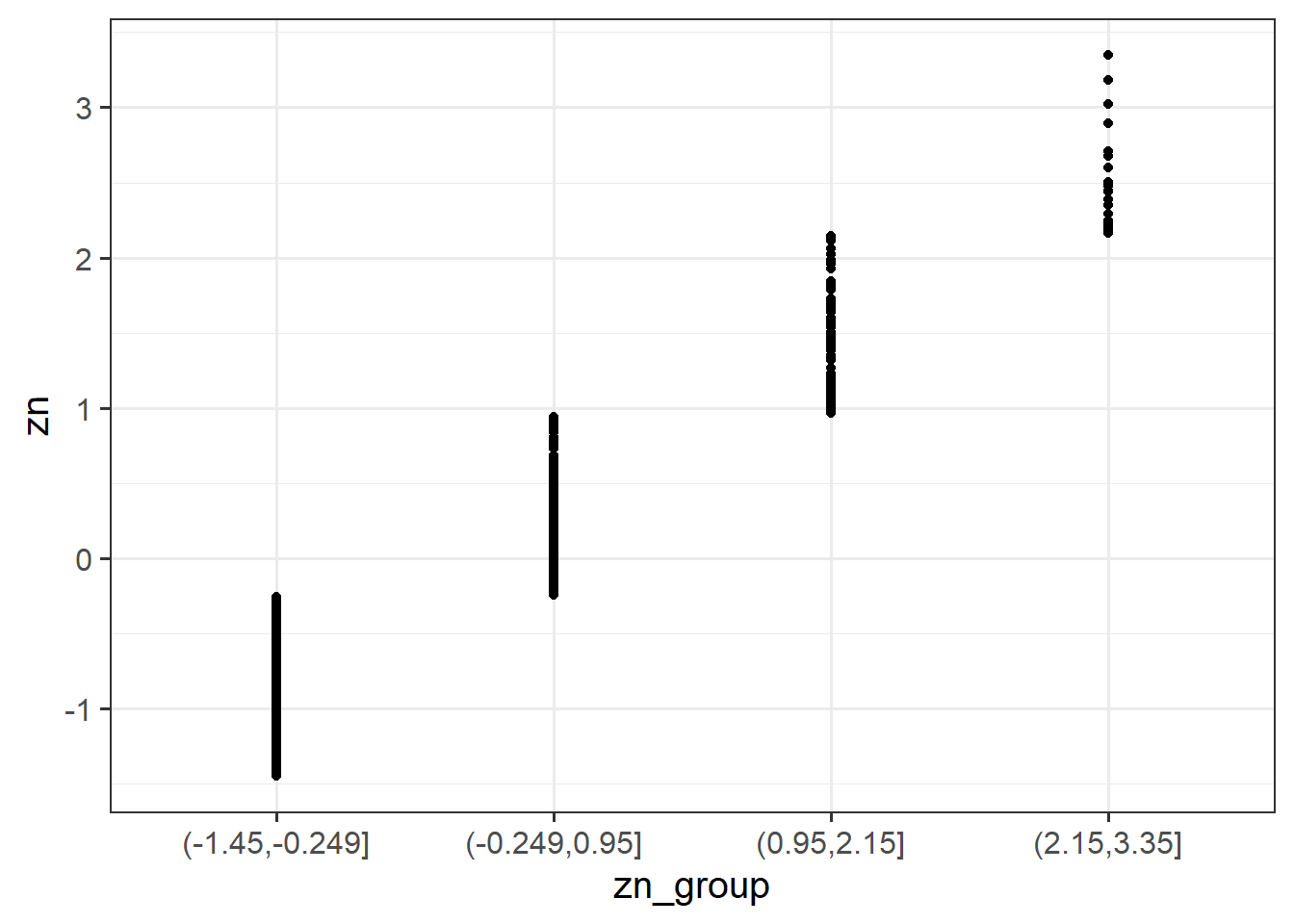

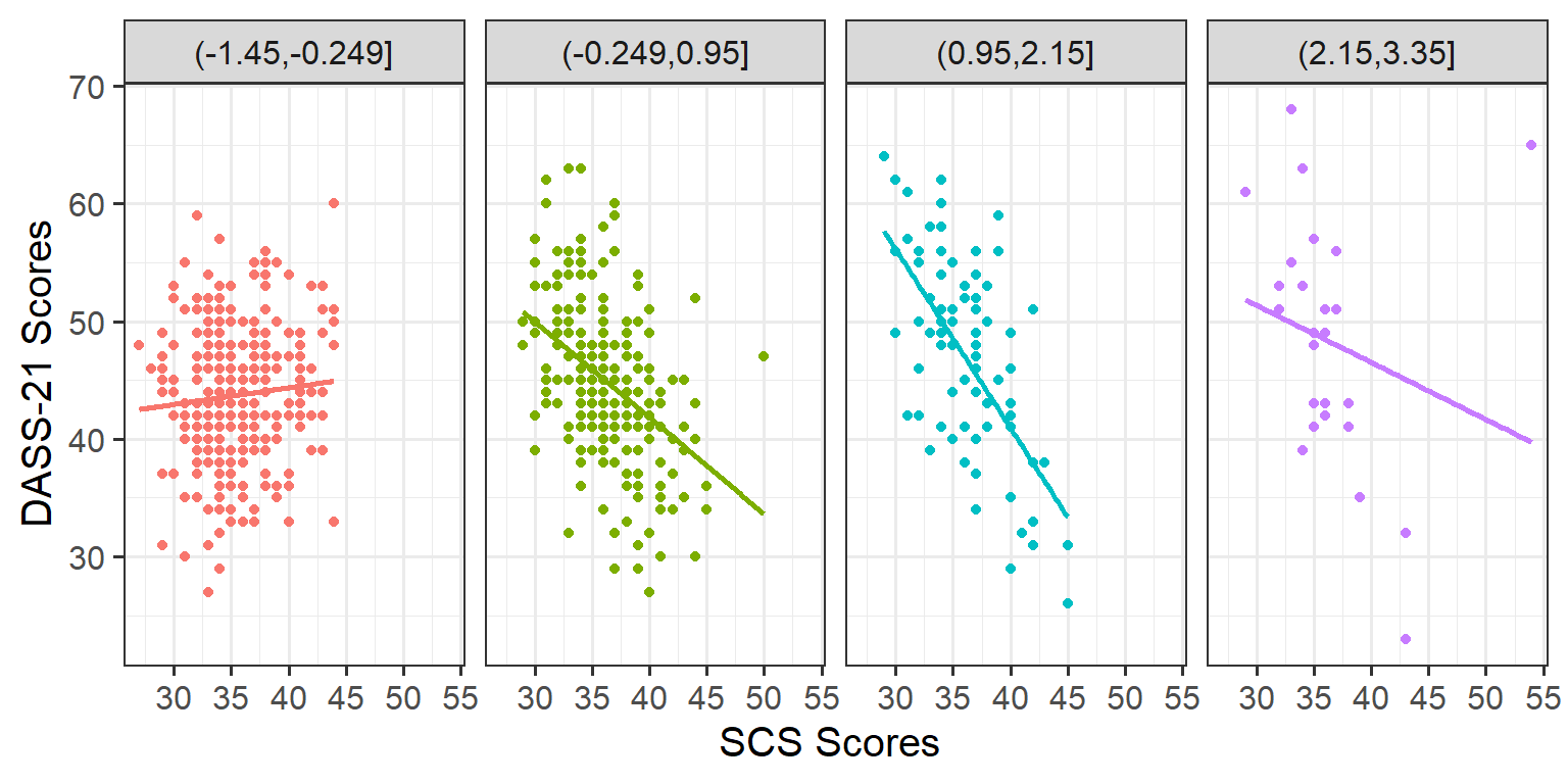
Plot the association between scores on the SCS and scores on the DASS-21, for each group of the variable we just created.

How does the pattern differ across groups? Does it suggest an interaction?

Hint

Rather than creating four separate plots, you might want to map some feature of the plot to the variable we created in the data, or make use of facet_wrap()/facet_grid().

Remember that you can specify geom_smooth() to add a trend line

Solution

ggplot(data = scs_study, aes(x = scs, y = dass, col = zn_group)) + 
  geom_point() + 
  geom_smooth(method='lm', se = FALSE) +
  facet_grid(~zn_group) +
  labs(x = "SCS Scores ", y = "DASS-21 Scores") +
  theme(legend.position = "none") # removes the legend

The association between SCS scores and DASS-21 scores appears to be different across these groups. For those with a relatively high Neuroticism score, the association seems stronger, while for those with a low Neuroticism score there is almost no discernible association.

This does suggest an interaction - the association of DASS-21 ~ SCS differs across the values of Neuroticism.

Visualising Interaction Terms

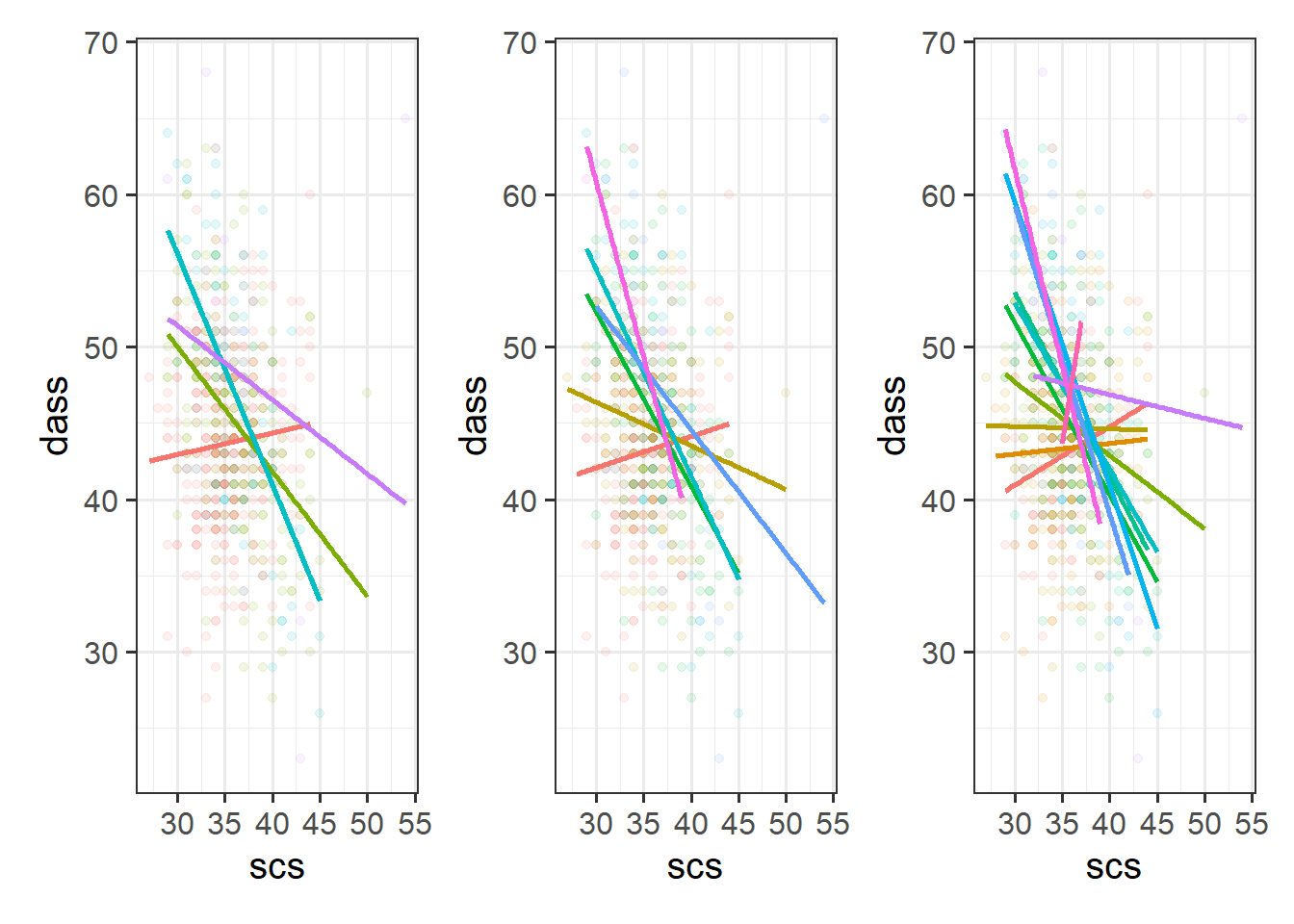
Cutting one of the explanatory variables up into groups essentially turns a numeric variable into a categorical one. We did this just to make it easier to visualise how an association differs across the values of another variable, because we can imagine a separate line for the association between SCS and DASS-21 scores for each of the groups of Neuroticism. However, in grouping a numeric variable like this we lose information. Neuroticism is measured on a continuous scale, and we want to capture how the association between SCS and DASS-21 differs across that continuum (rather than cutting it into chunks).

We could imagine cutting it into more and more chunks (see Figure 1), until what we end up with is an infinite number of lines - i.e., a three-dimensional plane/surface (recall that in for a multiple regression model with 2 explanatory variables, we can think of the model as having three-dimensions). The inclusion of the interaction term simply results in this surface no longer being necessarily flat. You can see this in Figure 2).

Figure 1: Separate regression lines DASS ~ SCS for Neuroticism when cut into 4 (left) or 6 (center) or 12 (right) groups.

Figure 2: 3D plot of regression surface with interaction. You can explore the plot in the figure below from different angles by moving it around with your mouse.

Question 4

Consider that Neuroticism has already been \(z\)-scored, but scs has not. To ensure that we can compare the effects of our estimates (and so they are both on meaningful scales), standardize the scs variable.

Hint

Recall the formula for the \(z\)-score: \[ z_x = \frac{x - \bar{x}}{s_x}, \qquad z_y = \frac{y - \bar{y}}{s_y} \]

Solution

# standardize scs score
scs_study <- 
  scs_study %>% 
    mutate(
      zscs = (scs-mean(scs))/sd(scs)
    )

Question 5

Fit your model (including the standardized variables) using lm(), and assign it as an object with the name “dass_mdl”.

Hint

When fitting a regression model in R with two explanatory variables A and B, and their interaction, these three are equivalent:

• y ~ A + B + A:B
• y ~ A + B + A*B
• y ~ A*B

Solution

#fit interaction model
dass_mdl <- lm(dass ~  zscs*zn, data = scs_study)

#check model output
summary(dass_mdl)

Call:
lm(formula = dass ~ zscs * zn, data = scs_study)

Residuals:
    Min      1Q  Median      3Q     Max 
-16.301  -3.825  -0.173   3.733  45.777 

Coefficients:
            Estimate Std. Error t value Pr(>|t|)    
(Intercept)  44.9324     0.2405 186.807  < 2e-16 ***
zscs         -1.5691     0.2416  -6.495 1.64e-10 ***
zn            1.5798     0.2409   6.559 1.11e-10 ***
zscs:zn      -1.8332     0.2316  -7.915 1.06e-14 ***
---
Signif. codes:  0 '***' 0.001 '**' 0.01 '*' 0.05 '.' 0.1 ' ' 1

Residual standard error: 6.123 on 652 degrees of freedom
Multiple R-squared:  0.1825,    Adjusted R-squared:  0.1787 
F-statistic:  48.5 on 3 and 652 DF,  p-value: < 2.2e-16

Question 6

Interpret your coefficients in the context of the study.

Solution

Recall that we can obtain our parameter estimates using various functions such as summary(),coef(), coefficients(), etc.

coefficients(dass_mdl)

(Intercept)        zscs          zn     zscs:zn 
  44.932448   -1.569097    1.579769   -1.833169 

• \(\beta_0\) = (Intercept) = 44.93
  • The intercept, or predicted DASS-21 score for average SCS score (Mean = 0) and average Neuroticism score (Mean = 0).
• \(\beta_1\) = zscs = -1.57
  • The simple slope of SCS scores for average Nueroticism scores (Mean = 0).
  • For an individual with average Neuroticism levels, DASS-21 scores decreased by 1.57 standard deviations for every 1 standard deviation increase in SCS scores.
• \(\beta_2\) = zn = 1.58
  • The simple slope of Neuroticism for average SCS scores (Mean = 0).
  • For those with average SCS scores, DASS-21 scored increased by 1.58 for every 1 standard deviation increase in Neuroticism.
• \(\beta_3\) zscs:zn = -1.83
  • The interaction between SCS score and Neuroticism on DASS-21 Scores
  • For every 1 standard deviation increase in SCS scores, the association between Neuroticism and DASS-21 scores decreases by an additional 1.83 standard deviations.

Question 7

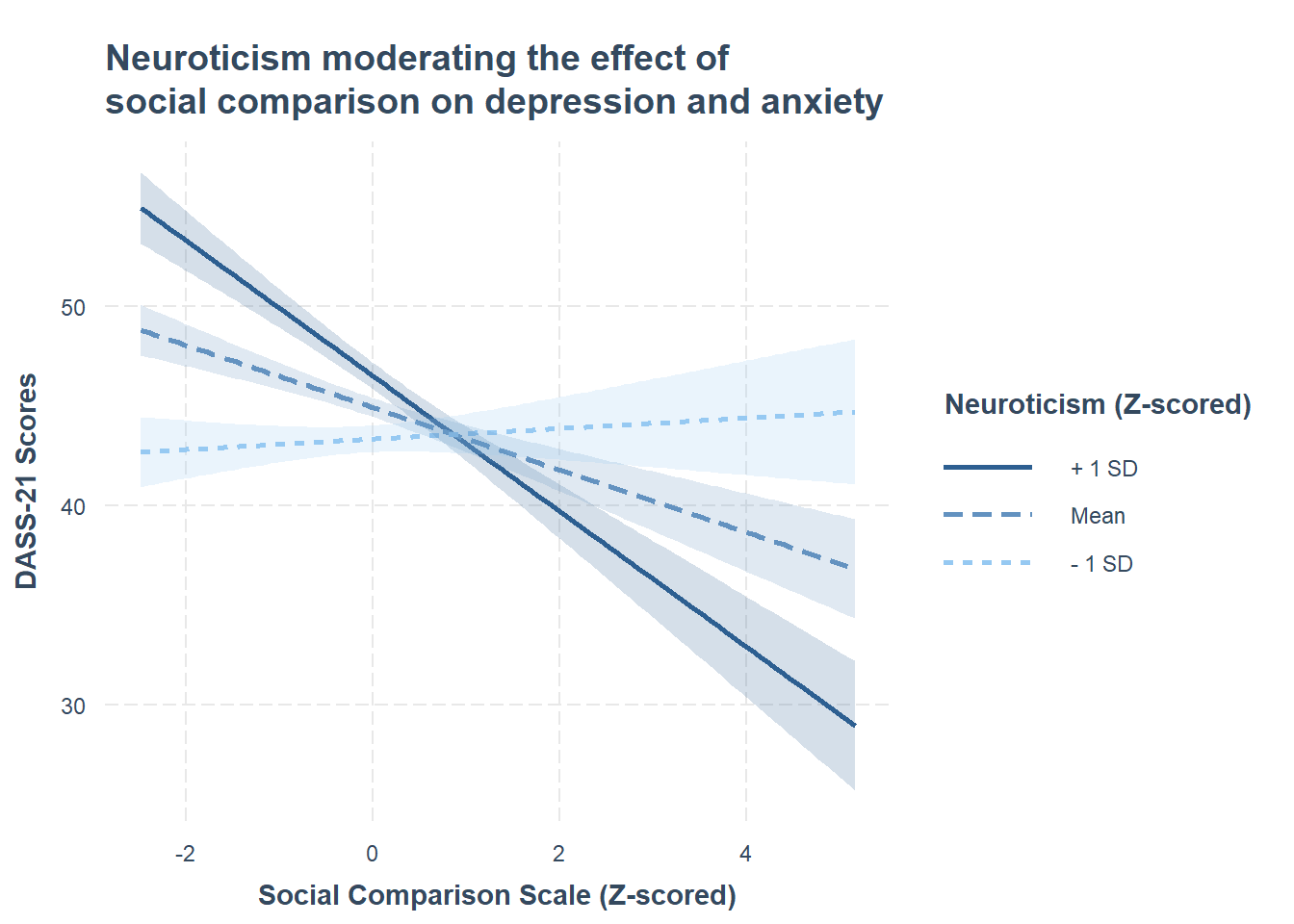
Using the probe_interaction() function from the interactions package, visualise the interaction effects from your model.

Try to summarise the interaction effects in a short and concise sentence.

Hint

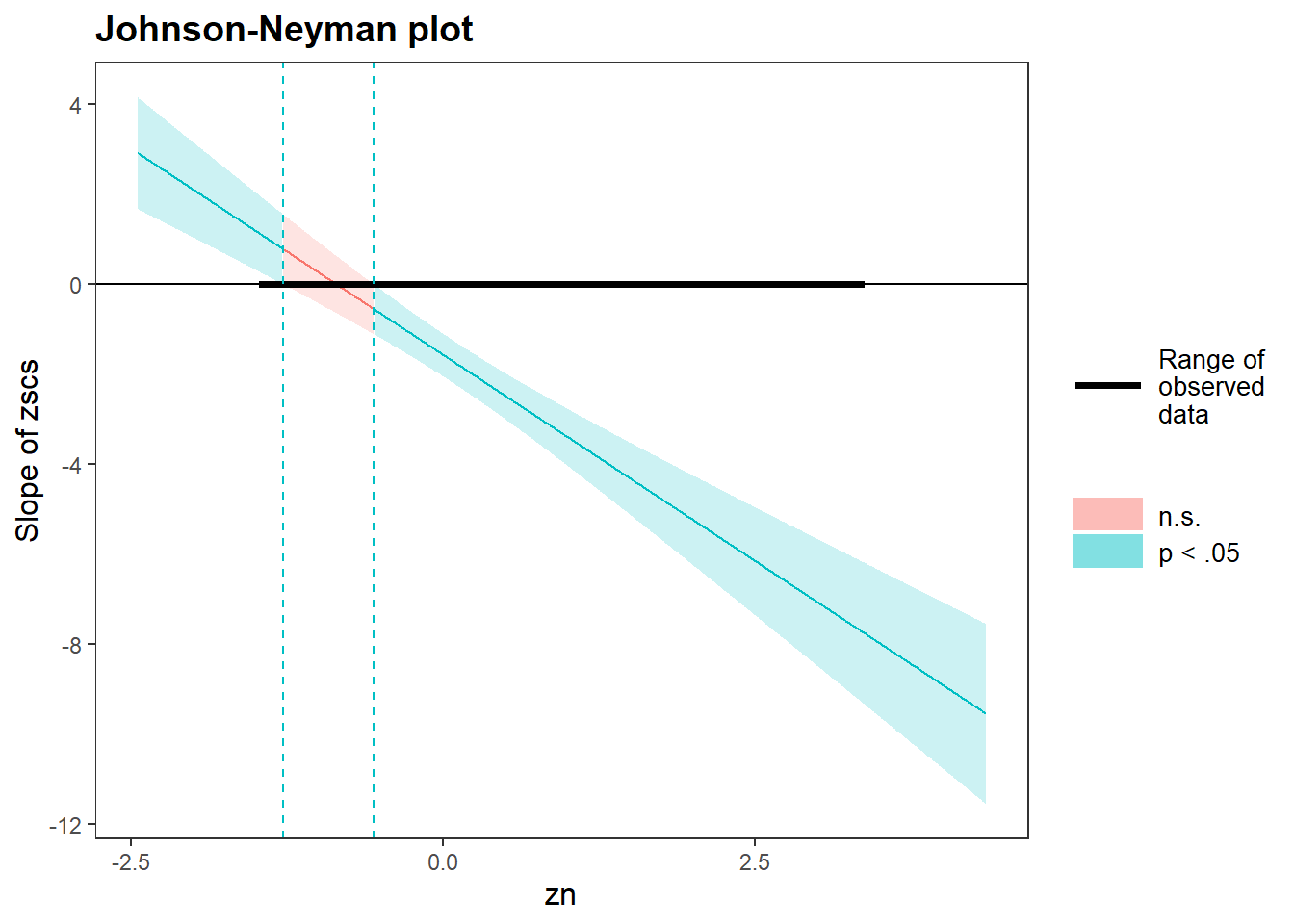
Because we are looking at a numeric x numeric interaction, we want to specify jnplot = T (see this weeks lecture, slides 17-21 for a worked example).

Remember to give your plot informative titles/labels. You, for example, likely want to give your plot:

• a clear and concise title (specify main.title =)
• axis labels with units or scale included (specify x.label = and y.label =)
• a legend title (specify legend.main =)

Solution

plt_dass_mdl <- probe_interaction(model = dass_mdl, 
                  pred = zscs, 
                  modx = zn, 
                  cond.int = T,
                  interval = T, 
                  jnplot = T,
                  main.title = "Neuroticism moderating the effect of\nsocial comparison on depression and anxiety",
                  x.label = "Social Comparison Scale (Z-scored)",
                  y.label = "DASS-21 Scores",
                  legend.main = "Neuroticism (Z-scored)")

Let’s look at the plot - to do so you need to call interactplot from your object plt_dass_mdl:

plt_dass_mdl$interactplot

Figure 3: Simple Sloes for +/- 1 SD and Mean Neuroticism Scores

The effect of SCS scores on DASS-21 scores was more negatively pronounced for those with higher Neuroticism scores.

Question 8

Conduct a simple slopes analysis.

Hint

If you wanted to see only the simple slopes or only the Johnson-Neyman plot, you could call $simslopes$slopes or simslopes$jnplot respectively from your object plt_dass_mdl.

Solution

plt_dass_mdl$simslopes

JOHNSON-NEYMAN INTERVAL 

When zn is OUTSIDE the interval [-1.28, -0.55], the slope of zscs is p <
.05.

Note: The range of observed values of zn is [-1.45, 3.35]

SIMPLE SLOPES ANALYSIS 

When zn = -1.000000e+00 (- 1 SD): 

                               Est.   S.E.   t val.      p
--------------------------- ------- ------ -------- ------
Slope of zscs                  0.26   0.35     0.76   0.45
Conditional intercept         43.35   0.34   127.47   0.00

When zn = -8.610271e-16 (Mean): 

                               Est.   S.E.   t val.      p
--------------------------- ------- ------ -------- ------
Slope of zscs                 -1.57   0.24    -6.50   0.00
Conditional intercept         44.93   0.24   186.81   0.00

When zn =  1.000000e+00 (+ 1 SD): 

                               Est.   S.E.   t val.      p
--------------------------- ------- ------ -------- ------
Slope of zscs                 -3.40   0.32   -10.59   0.00
Conditional intercept         46.51   0.34   136.52   0.00

Figure 4: Johnson-Neyman Plot

The Johnson-Neyman technique indicated that the association between DASS-21 scores and SCS was significant when Neuroticism scores were less than 1.28 standard deviations below the mean or more than -0.55 standard deviations above the mean.

Question 9

Provide key model results in a formatted table.

Hint

Use tab_model() from the sjPlot package.

Remember that you can rename your DV and IV labels by specifying dv.labels and pred.labels.

Solution

#create table for results
tab_model(dass_mdl,
          dv.labels = "DASS-21 Scores",
          pred.labels = c("zscs" = "Social Comparison Scale (Z-scored)",
                          "zn" = "Neuroticism (Z-scored)",
                          "zscs:zn" = "Social Comparison Scale (Z-scored): Neutoricism (Z-scored)"),
          title = "Regression table for DASS-21 model")

Table 2: Regression table for DASS-21 model

	DASS-21 Scores
Predictors	Estimates	CI	p
(Intercept)	44.93	44.46 – 45.40	<0.001
Social Comparison Scale (Z-scored)	-1.57	-2.04 – -1.09	<0.001
Neuroticism (Z-scored)	1.58	1.11 – 2.05	<0.001
Social Comparison Scale (Z-scored): Neutoricism (Z-scored)	-1.83	-2.29 – -1.38	<0.001
Observations	656
R2 / R2 adjusted	0.182 / 0.179

Question 10

Interpret your results in the context of the research question and report your model in full.

Make reference to the interaction plot and regression table.

Solution

Make sure to write your results up following APA guidelines:

Full regression results including 95% Confidence Intervals are shown in Table 2. The \(F\)-test for model utility was significant \((F(3,652) = 48.50, p<.001)\), and the model explained approximately 17.87% of the variability in DASS-21 scores.

There was a significant conditional association between DASS-21 Scores and SCS scores (Z-scored) (\(\beta\) = -1.57, SE = 0.24, \(p\) < .001), suggesting that for those with average Neuroticism scores (\(M\) = 0),DASS-21 scores decreased by 1.57 for every 1 standard deviation increase in SCS scores.

A significant conditional association was also evident between DASS-21 Scores and Neuroticism (Z-scored) (\(\beta\) = 1.58, SE = 0.24, \(p\) <.001), suggesting that for those with average SCS scores (\(M\) = 0), DASS-21 scores increased by 1.58 for every 1 standard deviation increase in Neuroticism.

The association between symptoms of depression and anxiety (DASS-21 scores) and social comparison was found to be dependent upon the level of Neuroticism, with a greater negative association between the two for those with high levels of Neuroticism (\(\beta\) = -1.83, SE = 0.23, \(p\) <.001). This buffering interaction suggested that for every standard deviation increase in SCS Scores, the negative influence of Neuroticism on DASS-21 scores was reduced by 1.83 standard deviations (see Figure 3). We further used the Johnson-Neyman technique to probe the interaction, and to identify regions of significance. We identified that Neuroticism values (z-scored) outside the range of -1.28 to -0.55 were significant (see Figure 4).

Therefore, we have evidence to reject the null hypothesis (that the effect of social comparison on symptoms of depression, anxiety and stress does not vary depending on level of Neuroticism).