Interactions 2

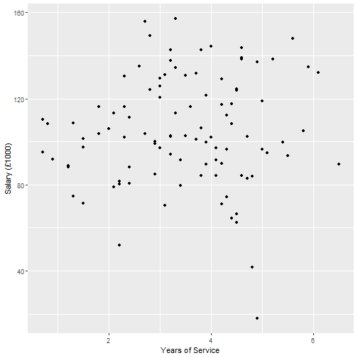
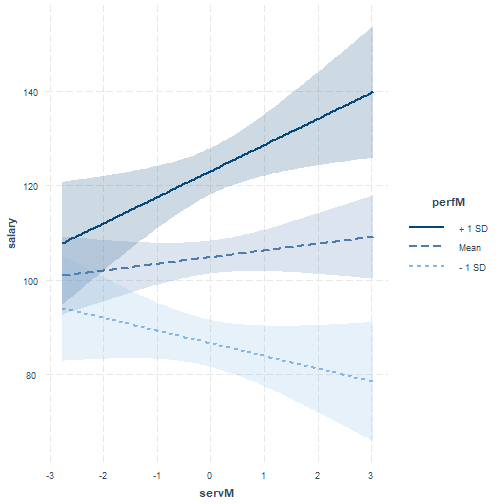
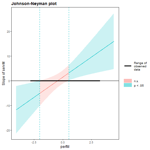
class: center, middle, inverse, title-slide

.title[
# <b>Interactions 2 </b>
]
.subtitle[
## Data Analysis for Psychology in R 2<br><br>
]
.author[
### dapR2 Team
]
.institute[
### Department of Psychology<br>The University of Edinburgh
]

---

# Weeks Learning Objectives
1. Understand the concept of an interaction.

2. Interpret interactions for between quantitative variables.

3. Visualize and probe interactions in R.

4. Recognise different forms of interaction.

---
#  General definition

+ When the effects of one predictor on the outcome differ across levels of another predictor.

+ Continuous-continuous interaction (**referred to as moderation**):
	+ The slope of the regression line between a continuous predictor and the outcome changes as the values of a second continuous predictor change.
	
+ Note interactions are symmetrical. We can talk about interaction of X with Z, or Z with X.

---
#  Lecture notation

`$$y_i = \beta_0 + \beta_1 x_{i} + \beta_2 z_{i} + \beta_3 xz_{i} + \epsilon_i$$`

+ Lecture notation:
  + `$y$` is a continuous outcome
  
  + `$x$` is a continuous predictor
  
  + `$z$` is a continuous predictor
  
  + `$xz$` is their product or interaction predictor

---
#  Interpretation: Continuous*Continuous

`$$y_i = \beta_0 + \beta_1 x_{i} + \beta_2 z_{i} + \beta_3 xz_{i} + \epsilon_i$$`

+ Lecture notation:
  
  + `$\beta_0$` = Value of `$y$` when `$x$` and `$z$` are 0
  
  + `$\beta_1$` = Effect of `$x$` (slope) when `$z$` = 0
  
  + `$\beta_2$` = Effect of `$z$` (slope) when `$x$` = 0
  
  +  `$\beta_3$` = Change in slope of `$x$` on `$y$` across values of `$z$` (and vice versa).
	    + Or how the effect of `$x$` depends on `$z$` (and vice versa)

---
#  Interpretation: Continuous*Continuous

`$$y_i = \beta_0 + \beta_1 x_{i} + \beta_2 z_{i} + \beta_3 xz_{i} + \epsilon_i$$`

+ Note, `$\beta_1$` and `$\beta_2$` and are referred to as conditional effects, **not as main effects** .
	
	+ They are the effects at the value 0 of the interacting variable.
	
	+ Main effects are typically assumed to be constant.
	
	+ For any `$\beta$` associated with a variable **not** included in the interaction, interpretation does not change.

---
#  Example: Continuous*Continuous

+ Conducting a study on how years of service and employee performance ratings predicts salary in a sample of managers.

`$$y_i = \beta_0 + \beta_1 x_{i} + \beta_2 z_{i} + \beta_3 xz_{i} + \epsilon_i$$`

+ `$y$` = Salary (unit = thousands of pounds ).

+ `$x$` = Years of service.

+ `$z$` = Average performance ratings.

---
#  Plot Salary and Service

.pull-left[

```r
salary2 %>%
  ggplot(., aes(x=serv, y=salary)) +
  geom_point() +
  labs(x = "Years of Service", 
       y = "Salary (£1000)")
```
]

.pull-right[
![](dapr2_07_interactions2_files/figure-html/unnamed-chunk-3-1.png)
]

---
#  Example: Continuous*Continuous

```
## 
## Call:
## lm(formula = salary ~ serv * perf, data = salary2)
## 
## Residuals:
##     Min      1Q  Median      3Q     Max 
## -43.008  -9.710  -1.068   8.674  48.494 
## 
## Coefficients:
##             Estimate Std. Error t value Pr(>|t|)    
## (Intercept)   87.920     16.376   5.369 5.51e-07 ***
## serv         -10.944      4.538  -2.412  0.01779 *  
## perf           3.154      4.311   0.732  0.46614    
## serv:perf      3.255      1.193   2.728  0.00758 ** 
## ---
## Signif. codes:  0 '***' 0.001 '**' 0.01 '*' 0.05 '.' 0.1 ' ' 1
## 
## Residual standard error: 17.55 on 96 degrees of freedom
## Multiple R-squared:  0.5404,	Adjusted R-squared:  0.5261 
## F-statistic: 37.63 on 3 and 96 DF,  p-value: 3.631e-16
```

???
+ General comments:
	+ The coefficients for service and the interaction are significant at nominal alpha = 0.05.
	+ R-squared suggests we have a good model
		+ Explains 54.04% variance.
	+ Difference in R-squared to adjusted is small (0.42%)

---
#  Example: Continuous*Continuous

.pull-left[

+ **Intercept**: a manager with 0 years of service and 0 performance rating earns £87,920

+ **Service**: for a manager with 0 performance rating, for each year of service, salary decreases by £10,940
  + slope when performance = 0
  
+ **Performance**: for a manager with 0 years service, for each point of performance rating, salary increases by £3,150.
  + slope when service = 0
  
+ **Interaction**: for every year of service, the relationship between performance and salary increases by £3250.

]

.pull-right[

```
##             Estimate Std. Error t value Pr(>|t|)
## (Intercept)    87.92      16.38    5.37     0.00
## serv          -10.94       4.54   -2.41     0.02
## perf            3.15       4.31    0.73     0.47
## serv:perf       3.25       1.19    2.73     0.01
```

]

???
+ What do you notice here?
+ 0 performance and 0 service are odd values
+ lets mean centre both, so 0 = average, and look at this again.

---
# Mean centering

```r
salary2 <- salary2 %>%
  mutate(
*   perfM = scale(perf, scale = F),
*   servM = scale(serv, scale = F)
  )

m2 <- lm(salary ~ servM*perfM, data = salary2)
```

---
# Mean centering

```
## 
## Call:
## lm(formula = salary ~ servM * perfM, data = salary2)
## 
## Residuals:
##     Min      1Q  Median      3Q     Max 
## -43.008  -9.710  -1.068   8.674  48.494 
## 
## Coefficients:
##             Estimate Std. Error t value Pr(>|t|)    
## (Intercept)  104.848      1.757  59.686  < 2e-16 ***
## servM          1.425      1.364   1.044  0.29890    
## perfM         14.445      1.399  10.328  < 2e-16 ***
## servM:perfM    3.255      1.193   2.728  0.00758 ** 
## ---
## Signif. codes:  0 '***' 0.001 '**' 0.01 '*' 0.05 '.' 0.1 ' ' 1
## 
## Residual standard error: 17.55 on 96 degrees of freedom
## Multiple R-squared:  0.5404,	Adjusted R-squared:  0.5261 
## F-statistic: 37.63 on 3 and 96 DF,  p-value: 3.631e-16
```

???

+ Pause the video. Take a few minutes to look at these results, vs the original model results 3 slides back.

+ What do we notice here?

1. The values of the coefficients have changed for service and performance
2. The p-value significance has changed
3. the interaction has stayed the same
4. the model coefficients have stayed the same

+ The coefficients change because these are the slopes at specific values of the other variable 0.
+ Remember with an interaction, the relationship changes as the values of the other variable change, so we expect this.
+ The p-values change, because the slope has changed. The null = 0, no effect. So if the slope gets bigger or smaller, the p-value will also change

---
#  Example: Continuous*Continuous

.pull-left[

+ **Intercept**: a manager with average years of service and average performance rating earns £104,850

+ **Service**: a manager with average performance rating, for every year of service, salary increases by £1,420
  + slope when performance = 0 (mean centered)
  
+ **Performance**: a manager with average years service, for each point of performance rating, salary increases by £14,450.
  + slope when service = 0 (mean centered)
  
+ **Interaction**: for every year of service, the relationship between performance and salary increases by £3,250.

]

.pull-right[

```
##             Estimate Std. Error t value Pr(>|t|)
## (Intercept)   104.85       1.76   59.69     0.00
## servM           1.42       1.36    1.04     0.30
## perfM          14.45       1.40   10.33     0.00
## servM:perfM     3.25       1.19    2.73     0.01
```

]

???
+ the values for `$\beta_1$` and `$\beta_2$` make a little more sense. We would expect service and performance increases to lead to increased pay.
+ However, there is an important point here. In the presence of a significant interaction, we tend not to interpret the conditional main effects.

+ This leads to the question of how do we interpret/understand the interaction.

+ and we will come to that next.

---
class: center, middle
# And breath

---
#  Plotting interactions

+ Simple slopes:
	+ **Regression of the outcome Y on a predictor X at specific values of an interacting variable Z.**
	
+ And we re-arranged such that:

`$$\hat{y} = (\beta_1 + \beta_3z)x + (\beta_2z + \beta_0)$$`

+ So all we need to do is select values of `$Z$`, or in our case, performance.
	+ This was easy when `$Z$` was binary (or categorical), we have a line for each group.
	+ Now we must select reasonable values.
	+ Norm is to take +/- 1SD and the mean value of `$Z$`.

---
#  Simple slope calculations

+ In the current data, the SD for performance is 1.26

+ We want to plot values for performance ( `$Z$` ) of -1.26, 0 and 1.26:

`$$\hat{salary} = (1.425 + (3.255*-1.26))service + ((14.445*-1.26) + 104.848)$$`

`$$\hat{salary} = (1.425 + (3.255*0))service + ((14.445*0) + 104.848)$$`

`$$\hat{salary} = (1.425 + (3.255*1.26))service + ((14.445*1.26) + 104.848)$$`

---
#  Probing interactions

+ We could plot these lines manually, but thankfully we have some useful

+ The linear model provides an omnibus test of the interaction effect.

+ But there may be specific hypotheses/questions about our simple slopes.

+ As such, we may want a way to test the significance of the slopes for specific values of the interacting variable.

---
#  `interactions`: Simple Slopes

.pull-left[

```r
library(interactions)
p_m2 <- probe_interaction(m2, 
                  pred = servM, 
                  modx = perfM, 
                  cond.int = T,
                  interval = T, 
                  jnplot = T)
```

]

.pull-right[

```r
p_m2$interactplot
```

![](dapr2_07_interactions2_files/figure-html/unnamed-chunk-10-1.png)

]

---
#  `interactions`: Simple Slopes

+ From the same function, we can look at the significance of the slopes:

```r
p_m2$simslopes$slopes
```

```
##   Value of perfM      Est.     S.E.      2.5%    97.5%    t val.          p
## 1  -1.263313e+00 -2.687136 1.877723 -6.414387 1.040114 -1.431061 0.15565998
## 2   1.776357e-16  1.424880 1.364229 -1.283094 4.132854  1.044458 0.29889653
## 3   1.263313e+00  5.536896 2.177515  1.214564 9.859229  2.542760 0.01259677
```

---
#  Probing interactions

+ Note that our simple slopes analysis requires us to pick-a-point of `$Z$` at which we test the slope.
	+ Sometimes, we may not have a particular reason to choose any particular value.
	+ That has led to a default being to choose the mean of Z, and +1 and -1 standard deviation from the mean (i.e. low-average-high).
	+ If we do not know what values to choose, we may want a more general approach.
	
+ Cue regions of significance.
	+ Region of significance analysis identifies the thresholds (values of `$Z$`) at which the regression of `$Y$` on `$X$` changes from non-significance to significance.

---
#  `interactions`: Simple Slopes

.pull-left[
+ Using the same object, we can look at regions of significance.

+ The function provides a plot ->

+ And text interpretation:

> When perfM is OUTSIDE the interval [-2.01, 0.53], the slope of servM is p < .05. Note: The range of observed values of perfM is [-2.80, 3.20]
]

.pull-right[
![](dapr2_07_interactions2_files/figure-html/unnamed-chunk-12-1.png)
]

---
#  `interactions`: Simple Slopes

.pull-left[
+ y-axis shows the conditional slopes of the effect of service ( `$x$` )
+ x-axis shows values of performance ( `$z$` )
+ Horizontal black line is at conditional slope = 0 (i.e. the null hypothesis)
+ The shaded area is the point-wise confidence interval for the simple slopes
  + In other words, it is showing the significance test.
  + If the shaded area crosses the horizontal black line, the the 95% CI includes 0.
+ The vertical dashed blue lines show the interval where the 95% CI's include 0.

]

.pull-right[
![](dapr2_07_interactions2_files/figure-html/unnamed-chunk-13-1.png)
]

---
class: center, middle
# Question break

---
#  Types of interaction

+ Ordinal:
	+ Lines do not cross within the plausible range of measurement of `$x$`.
	+ Rank order of one predictor is maintained across levels of another.
	+ More common in observational studies.

+ Disordinal :
	+ Line cross within the plausible range of measurement of `$x$`.
	+ Rank order of one predictor is not maintained across levels of another.
	+ More common in experimental work.

---
#  Locating a crossing point

`$$y_i = \beta_0 + \beta_1 x_{i} + \beta_2 z_{i} + \beta_3 xz_{i} + \epsilon_i$$`

+ For `$X$` (service), the cross point is:

`$$\frac{-\beta_2}{\beta_3}$$`

+ For `$Z$` (performance), the cross point is:

`$$\frac{-\beta_1}{\beta_3}$$`

+ In both cases it is clear that the cross point is dependent on the relative magnitudes of the first-order effect to the high-order (interaction) effect.

---
#  Locating a crossing point

.pull-left[
+ Calculations from `m2`.

+ For Performance:

`$$\frac{-1.425}{3.255} = -0.44$$`

+ For Service:

`$$\frac{-14.445}{3.255} = -4.44$$`

]

.pull-right[

![](dapr2_07_interactions2_files/figure-html/unnamed-chunk-14-1.png)

]

---
#  Types of interactions

<table class="table" style="font-size: 18px; margin-left: auto; margin-right: auto;">
 <thead>
  <tr>
   <th style="text-align:left;"> TYPE </th>
   <th style="text-align:left;"> B1 </th>
   <th style="text-align:left;"> B2 </th>
   <th style="text-align:left;"> B3 </th>
   <th style="text-align:left;"> DESCRIPTION </th>
  </tr>
 </thead>
<tbody>
  <tr>
   <td style="text-align:left;"> Synergistic </td>
   <td style="text-align:left;"> + ve </td>
   <td style="text-align:left;"> + ve </td>
   <td style="text-align:left;"> + ve </td>
   <td style="text-align:left;"> Enhancing effect. Interaction produces a bigger change than expected from additive model. Example: Alcohol*depressant drug effects on mood. </td>
  </tr>
  <tr>
   <td style="text-align:left;">  </td>
   <td style="text-align:left;"> - ve </td>
   <td style="text-align:left;"> - ve </td>
   <td style="text-align:left;"> - ve </td>
   <td style="text-align:left;">  </td>
  </tr>
  <tr>
   <td style="text-align:left;"> Antagonistic </td>
   <td style="text-align:left;"> + ve </td>
   <td style="text-align:left;"> + ve </td>
   <td style="text-align:left;"> - ve </td>
   <td style="text-align:left;"> Diminishing returns. The strength of the combined effect weakens as the level of variables increases. Example: IQ*Conscientiousness effect on school performance. </td>
  </tr>
  <tr>
   <td style="text-align:left;">  </td>
   <td style="text-align:left;"> - ve </td>
   <td style="text-align:left;"> - ve </td>
   <td style="text-align:left;"> + ve </td>
   <td style="text-align:left;">  </td>
  </tr>
  <tr>
   <td style="text-align:left;"> Buffering </td>
   <td style="text-align:left;"> + ve </td>
   <td style="text-align:left;"> - ve </td>
   <td style="text-align:left;"> +/- ve </td>
   <td style="text-align:left;"> One variable weakens the effect of the other. The direction of the buffering is driven by the sign of the coefficient for the interaction. Example: Neuroticism*Conscientiousness effect on health </td>
  </tr>
  <tr>
   <td style="text-align:left;">  </td>
   <td style="text-align:left;"> - ve </td>
   <td style="text-align:left;"> + ve </td>
   <td style="text-align:left;"> +/- ve </td>
   <td style="text-align:left;">  </td>
  </tr>
</tbody>
</table>

---
#  Higher order terms (Non-linear effects)

+ The interaction equation:

`$$y_i = \beta_0 + \beta_1 x_{i} + \beta_2 z_{i} + \beta_3 xz_{i} + \epsilon_i$$`

+ We have noted for a continuous*continuous interaction this is a non-linear effect.

+ We have spoken about non-linearity in the context of model assumptions.
	+ Does this mean we can have other non-linear effects?
	+ Yes, and it looks a lot like an interaction.

+ The equation with a non-linear term for `$X$`:

`$$y_i = \beta_0 + \beta_1 x_{i} + \beta_2 z_{i} + \beta_3 xx_{i} + \epsilon_i$$`

`$$y_i = \beta_0 + \beta_1 x_{i} + \beta_2 z_{i} + \beta_3 x_{i}^2 + \epsilon_i$$`

---
#  How do we know to include non-linear?

+ Theory
	+ Power for non-linear (higher order, interaction) effects is usually low (see final slides).
	+ This, and other features of data (e.g. skew), can lead to spurious interactions.
	+ So the best plan is not to go looking for them unless there is solid theory. But?

+ Sometimes data speaks up and let?s us know something may be misspecified in our models.
	+ E.g. evidence for non-linearity in our assumption checks.
	+ Inclusion of higher-order/interaction terms can help resolve issues with violated model assumptions (linearity & heteroscedasticity).

---
#  Power and interactions

+ Statistical power for identifying interactions is generally low.

+ This means that both Type I and Type II error rates are increased.
	+ We may fail to reject the null when we should.
	+ We may reject the null when we should not.

+ With low power there is also a tendency for effects to be over estimated.

+ What does all this mean?
	+ If you identify an interaction in an observational study with low N, be **very** cautious in your interpretation.
	+ What is low N? We will talk more about this in the last week.

---
# Summary of today

+ Interpreting continuous-continuous (quant-quant) interactions

+ Considered the importance of scale and centering

+ Calculated and visualized simple slopes for continuous variables

+ Define types of interactions based on patterns of coefficients and crossing points

+ Briefly linked interactions to the broader estimation on non-linear effects

---
class: center, middle
# Thanks for listening!