Testing and Evaluating LM

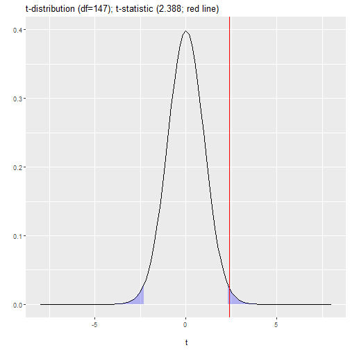
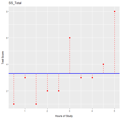
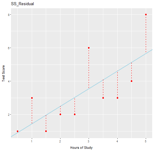
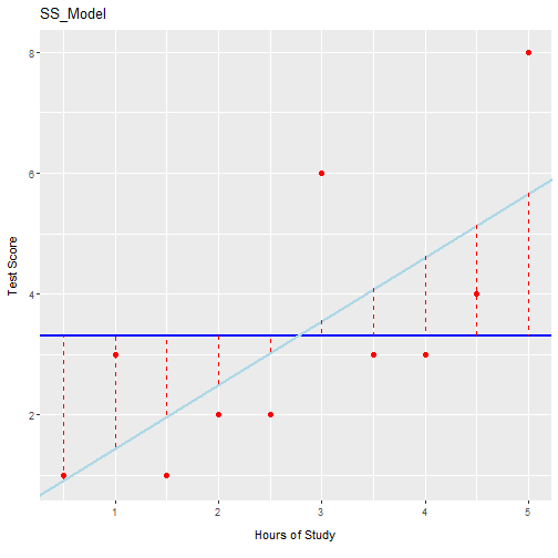
class: center, middle, inverse, title-slide

.title[
# Testing and Evaluating LM
]
.subtitle[
## Data Analysis for Psychology in R 2 
]
.author[
### dapR2 Team
]
.institute[
### Department of Psychology The University of Edinburgh
]

---

# Week's Learning Objectives
1. Understand how to interpret significance tests for `$\beta$` coefficients.
2. Understand how to calculate the interpret `$R^2$` and adjusted- `$R^2$` as a measure of model quality.
3. Be able to locate each of these tests in R `lm` model output.

---
# Recap
+ Last week we introduced the general linear model equation:

`$$y_i = \beta_0 + \beta_1 x_{i} + \epsilon_i$$`

+ And we ran an example concerning test scores:

`$$score_i = \beta_0 + \beta_1 hours_{i} + \beta_2 motivation_{i} + \epsilon_i$$`

+ And we looked at how to run this model in R:

```r
lm(score ~ hours + motivation, data = test_study2)
```

---
# Evaluating our model
+ At this point, we have estimated values for the key parameters of our model ( `$\beta$`s ).

+ Now we have to think about how we evaluate the model.

+ There are three ways to think about evaluation:

1. Evaluating the individual coefficients
  2. Evaluating the overall model quality
  3. Evaluating the model assumptions (later in the course)

+ Before accepting a set of results, it is important to consider all three of these aspects of evaluation.

???
Important to really emphasize this is a package of information and we want it all before we decide to accept our model.

---
#  Significance of individual effects 
+ A general way to ask this question would be to state:

> **Is our model model informative about the relationship between X and Y?**

+ In the context of our example from last lecture, we could ask,

> **Is study time a useful predictor of test score?**

+ The above is a research question/hypothesis. As we have done before, we need to turn this into a testable statistical hypothesis.

---
#  Evaluating individual predictors 
+ Steps in hypothesis testing:

--
  + Research questions
    
--
  
  + Statistical hypothesis
    
--
  
  + Define the null
    
--
  
  + Calculate an estimate of effect of interest.
  
--
  
  + Calculate an appropriate test statistic.
    
--
  
  + Evaluate the test statistic against the null.

---
# Research question and hypotheses

+ **Research questions** are statements of what we intend to study.

+ A good question defines:

+ Constructs under study
  + the relationship being tested
  + A direction of relationship
  + target populations etc.

> **Does increased study time improve test scores in school age children?**

+ **Statistical hypotheses** are testable mathematical statements.

+ In typical testing in Psychology, we define have a **null ( `$H_0$` )** and an **alternative ( `$H_1$` )** hypothesis.
  + `$H_0$` is precise, and states a specific value for the effect of interest.
  + `$H_1$` is not specific, and simply says "something else other than the null is more likely"

---
# Statistical significance: Overview

+ Remember, we only ever test the null.

+ We select a significance level, `$\alpha$` (typically .05)

+ Then we calculate the `$p$`-value associated with our test statistic (here `$\beta$` )

+ If the associated `$p$` is smaller, then we **reject** the null.

+ If it is larger, then we **fail to reject** the null.

---
# Our results

```r
performance <- lm(score ~ hours + motivation, data = test_study2); summary(performance)
```

```
## 
## Call:
## lm(formula = score ~ hours + motivation, data = test_study2)
## 
## Residuals:
## Min 1Q Median 3Q Max 
## -12.9548 -2.8042 -0.2847 2.9344 13.8240 
## 
## Coefficients:
## Estimate Std. Error t value Pr(>|t|) 
## (Intercept) 6.86679 0.65473 10.488 <2e-16 ***
## hours 1.37570 0.07989 17.220 <2e-16 ***
## motivation 0.91634 0.38376 2.388 0.0182 * 
## ---
## Signif. codes: 0 '***' 0.001 '**' 0.01 '*' 0.05 '.' 0.1 ' ' 1
## 
## Residual standard error: 4.386 on 147 degrees of freedom
## Multiple R-squared: 0.6696,	Adjusted R-squared: 0.6651 
## F-statistic: 148.9 on 2 and 147 DF, p-value: < 2.2e-16
```

---
class: center, middle
# A brief pause

**Any questions before we look at this process in a little more detail**

---
# Defining null

+ Conceptually:
	+ If `$x$` yields no information on `$y$`, then `$\beta_1 = 0$`
	
+ **Why would this be the case?**

--
	+ `$\beta$` gives the predicted change in `$y$` for a unit change in `$x$`.
	+ If `$x$` and `$y$` are unrelated, then a change in `$x$` will not result in any change to the predicted value of `$y$`
	+ So for a unit change in `$x$`, there is no (=0) change in `$y$`.
	
+ We can state this formally as a null and alternative:

`$$H_0: \beta_1 = 0$$`
`$$H_1: \beta_1 \neq 0$$`

???
+ For the null to be testable, we need to formally define it. 
+ Point out here the difference in the specificity of the hypotheses. `$H_0$` is that the `$b_1$` takes a specific value. `$H_1$` is that `$b_1$` has some value that is not this specific value. i..e one is directly testable, the other is not.

---
# Point estimate and test statistic

+ We have already seen how we calculate `$\hat \beta_1$`.

+ The associated test statistic to for `$\beta$` coefficients is a `$t$`-statistic

`$$t = \frac{\hat \beta}{SE(\hat \beta)}$$`

+ where

+ `$\hat \beta$` = any `$\beta$` coefficient we have calculated
  + `$SE(\hat \beta)$` = standard error of `$\beta$`

+ **Recall** that the standard error describes the spread of the sampling distribution.
  + The standard error (SE) provides a measure of sampling variability
  + Smaller SE's suggest more precise estimate (=good)
  
???
+ brief reminders on test statistics
  + every quantity we wish to calculate a significance test for needs an test statistic.
  + the test statistic is a value that has a known sampling distribution
+ If sampling distribution is unfamiliar, again, recap the hypothesis testing material

---
# Lets look at the output from `lm` again

```r
summary(performance)
```

---
# And work out the `$t$`-values

+ We can check the value for `motivation` first:

`$$t = \frac{\hat \beta_1}{SE(\hat \beta_1)} = \frac{0.9163}{0.3838} = 2.388 (3dp)$$`

+ Check `hours` in your own time.

+ So we know where the `$\beta$` values come from, and we have just seen `$t$`, what about the `$SE$` and `$p$`

---
#  SE( `$\hat \beta_1$` )

+ The formula for the standard error of the slope is:

`$$SE(\hat \beta_j) = \sqrt{\frac{ SS_{Residual}/(n-k-1)}{\sum(x_{ij} - \bar{x_{j}})^2(1-R_{xj}^2)}}$$`
+ Where:
	+ `$SS_{Residual}$` is the residual sum of squares
	+ `$n$` is the sample size
	+ `$k$` is the number of predictors
	+ `$x_{ij}$` is the observed value of a predictor ( `$j$` ) for an individual ( `$i$` )
	+ `$\bar{x_{ij}$` is the mean of a predictor
	+ `$(1 - R_{xj}^2)$` is the multiple correlation coefficient of the predictors

+ `$(1 - R_{xj}^2)$` captures to degree to which all of our predictors are related.
  + For simple linear models, this = 0 as there is only 1 predictor
  
---
# SE( `$\hat \beta_1$` )

`$$SE(\hat \beta_j) = \sqrt{\frac{ SS_{Residual}/(n-k-1)}{\sum(x_{ij} - \bar{x_{j}})^2(1-R_{xj}^2)}}$$`  
+ We want our `$SE$` to be smaller - this means our estimate is precise

+ Examining the above formula we can see that:
	+ `$SE$` is smaller when residual variance ( `$SS_{residual}$` ) is smaller
	+ `$SE$` is smaller when sample size ( `$N$` ) is larger
	+ `$SE$` is larger when the number of predictors ( `$k$` ) is larger
	+ `$SE$` is larger when a predictor is strongly correlated with other predictors ( `$R_{xj}^2$` )

+ So all we have left is `$p$`

???
+ Well return to this later when we discuss multi-collinearity issues

---
# Sampling distribution for the null

+ Now we have our `$t$`-statistic, we need to evaluate it.

+ For that, we need sampling distribution for the null.

+ For `$\beta$`, this is a `$t$`-distribution with `$n-k-1$` degrees of freedom.
	+ Where `$k$` is the number of predictors, and the additional -1 represents the intercept.

+ So in our example:
  + n = 150
  + k = 2
  + 150 - 2 - 1 = 147

---
#  A decision about the null 
+ So we have a `$t$`-value associated with our `$\beta$` coefficient.
	+ t = 2.388

+ And we know we will evaluate it against a `$t$`-distribution with 147 df.

+ As with all tests we need to set our `$\alpha$`.
	+ Let's take 0.05 two tailed.

+ Now we need a critical value to compare our observed `$t$`-value to.

---
# Visualize the null

.pull-left[
![](dapr2_03_testinglm_files/figure-html/unnamed-chunk-6-1.png)

]

.pull-right[

+ Critical value and `$p$`-value:

```r
tibble(
  LowerCrit = round(qt(0.025, 147), 3),
  UpperCrit = round(qt(0.975, 147), 3),
  Exactp = (1 - pt(2.388, 147)) * 2
)
```

```
## # A tibble: 1 × 3
## LowerCrit UpperCrit Exactp
## <dbl> <dbl> <dbl>
## 1 -1.98 1.98 0.0182
```

]

???
+ discuss this plot.
+ remind them of 2-tailed
+ areas
+ % underneath each end
+ comment on how it would be different one tailed
+ remind about what X is, thus where the line is

---
#  Confidence intervals for `$\beta$`
+ We can also compute confidence intervals for `$\hat \beta$`
+ The `$100 (1 - \alpha)$`, e.g., 95%, confidence interval for the slope is:

`$$\hat \beta_1 \pm t^* \times SE(\hat \beta_1)$$`

+ So, 95% confidence interval for in our example for the effect of `motivation` would be:

```r
tibble(
  LowerCI = round(0.91634 - (qt(0.975, 147) * 0.38376), 3),
  UpperCI = round(0.91634 + (qt(0.975, 147)* 0.38376), 3)
)
```

```
## # A tibble: 1 × 2
## LowerCI UpperCI
## <dbl> <dbl>
## 1 0.158 1.68
```

+ The confidence interval of 0.158 to 1.675 does not include zero, 
 + Therefore, we can conclude that **motivation is a statistically significant predictor of test scores** ( `$p < .05$`).

---
# `confint` function

+ We can get confidence intervals for our models more easily than this:

```r
confint(performance)
```

```
##                 2.5 %   97.5 %
## (Intercept) 5.5728881 8.160686
## hours       1.2178208 1.533576
## motivation  0.1579477 1.674729
```

---
# Where are we up to...

```r
performance <- lm(score ~ hours + motivation, data = test_study2)
summary(performance)
```

---
class: center, middle
# Time for a break! Questions

---
#  Quality of the overall model 
+ When we measure an outcome ( `$y$` ) in some data, the scores will vary (we hope).
  + Variation in `$y$` = total variation of interest.

+ The aim of our linear model is to build a model which describes `$y$` as a function of `$x$`.
	+ That is we are trying to explain variation in `$y$` using `$x$`.

+ But it won't explain it all.
  + What is left unexplained is called the residual variance.

+ So we can breakdown variation in our data based on sums of squares as;

`$$SS_{Total} = SS_{Model} + SS_{Residual}$$`

---
#  Coefficient of determination 
+ One way to consider how good our model is, would be to consider the proportion of total variance our model accounts for.

`$$R^2 = \frac{SS_{Model}}{SS_{Total}} = 1 - \frac{SS_{Residual}}{SS_{Total}}$$`

+ `$R^2$` = coefficient of determination

+ Quantifies the amount of variability in the outcome accounted for by the predictors.
  + More variance accounted for, the better.
  + Represents the extent to which the prediction of `$y$` is improved when predictions are based on the linear relation between `$x$` and `$y$`.

+ Let's see how it works.
  + To do so, we need to calculate the different sums of squares.

---
# Total Sum of Squares

.pull-left[
+ Sums of squares quantify difference sources of variation.

`$$SS_{Total} = \sum_{i=1}^{n}(y_i - \bar{y})^2$$`

+ Squared distance of each data point from the mean of `$y$`.

+ Mean is our baseline.

+ Without any other information, our best guess at the value of `$y$` for any person is the mean.

]

.pull-right[

![](dapr2_03_testinglm_files/figure-html/unnamed-chunk-11-1.png)

]

---
# Residual sum of squares

.pull-left[
+ Sums of squares quantify difference sources of variation.

`$$SS_{Residual} = \sum_{i=1}^{n}(y_i - \hat{y}_i)^2$$`

+ Which you may recognise.

+ Squared distance of each point from the predicted value.
]

.pull-right[

![](dapr2_03_testinglm_files/figure-html/unnamed-chunk-12-1.png)

]

---
# Model sums of squares

.pull-left[
+ Sums of squares quantify difference sources of variation.

`$$SS_{Model} = \sum_{i=1}^{n}(\hat{y}_i - \bar{y})^2$$`

+ That is, it is the deviance of the predicted scores from the mean of `$y$`.

+ But it is easier to simply take:

`$$SS_{Model} = SS_{Total} - SS_{Residual}$$`

]

.pull-right[

![](dapr2_03_testinglm_files/figure-html/unnamed-chunk-13-1.png)

]

---
# Values in our sample
+ In the current example, these values are:

+ `$SS_{total}$` = 8556.06
  + `$SS_{residual}$` = 2826.83
  + `$SS_{model}$` = 5729.23

+ In the LEARN folder there is a document which shows the calculations from the raw data

---
#  Coefficient of determination 
+ Now we can finally come back to `$R^2$`.

`$$R^2 = 1 - \frac{SS_{Residual}}{SS_{Total}}$$`

+ Or

`$$R^2 = \frac{SS_{Model}}{SS_{Total}}$$`

+ So in our example:

`$$R^2 = \frac{SS_{Model}}{SS_{Total}} = \frac{5729.23}{8556.06} = 0.6695$$`

+ ** `$R^2$` = 0.6695 means that 66.95% of the variation in test scores is accounted for by hours of revision and student motivation.**

---
#  Our example

```r
summary(performance)
```

???
As at the end of last session, we can check this against the R-output:
Be sure to flag small amounts of rounding difference from working through "by hand" and so presenting to less decimal places.

---
#  Adjusted `$R^2$` 
+ We can also compute an adjusted `$R^2$` when our `lm` has 2+ predictors.
  + `$R^2$` is an inflated estimate of the corresponding population value

+ Due to random sampling fluctuation, even when `$R^2 = 0$` in the population, it's value in the sample may `$\neq 0$`

+ In **smaller samples** , the fluctuations from zero will be larger on average

+ With **more IVs** , there are more opportunities to add to the positive fluctuation

`$$\hat R^2 = 1 - (1 - R^2)\frac{N-1}{N-k-1}$$`

+ Adjusted `$R^2$` adjusts for both sample size ( `$N$` ) and number of predictors ( `$k$` )

---
#  In our example

```r
summary(performance)
```

---
#  In our example

+ **Based on adjusted R-squared, hours studying and student motivation explain 66.5% of the variance in test scores**

+ As the sample size is large and the number of predictors small, unadjusted ( 0.67 ) and adjusted R-squared ( 0.665 ) are similar.

---
class: center, middle
# Any questions...

---
# Summary

+ Key take homes:
  1. We have an inferential test, based on a `$t$`-distribution, for the significance of `$\beta$`.
  2. We are more likely to find a significant effect when we have picked good variables (smaller residual SS) and we have a large sample.
  3. We can assess the degree to which our model explains variance in the outcome based on `$R^2$`
  4. When we have multiple predictors, we can use the adjusted `$R^2$` to account for the random fluctuations due to the model being more complex.
  
+ Next week we will look at model comparisons and standardization of coefficients.

---
class: center, middle
# Thanks for listening!