Sample Size and Power Analysis
LEARNING OBJECTIVES
- Understand differences between Type I and Type II errors
- Understand how varying factors can influence power
- Be able to conduct power analyses using the
pwrpackage
Before describing and analysing data, you have to collect data. If you’re lucky enough, someone else will have collected the data you need and these will be provided to you, but other times you have to collect the data needed to answer your research question yourself. This leads to some experimental design issues, such as how big should the sample be?
This is exactly the question that we will be answering this week discussing power analysis.
Power analysis lets you determine how many subjects are needed for your study or, conversely, whether your study is any worth pursuing if you can only afford to sample \(n\) units.
Notation
In the following, the symbol \(P()\) denotes the probability of whatever is within the parentheses.
Errors and Power in Hypothesis Testing
When testing an hypothesis, we reach one of the following two decisions:
- failing to reject \(H_0\) as the evidence against it is not sufficient
- rejecting \(H_0\) as we have enough evidence against it
However, irrespective of our decision, the underlying truth can either be that
- \(H_0\) is actually false
- \(H_0\) is actually true
Hence, we have four possible outcomes following an hypothesis test:
- We failed to reject \(H_0\) when it was true, meaning we made a Correct decision
- We rejected \(H_0\) when it was false, meaning we made a Correct decision
- We rejected \(H_0\) when it was true, committing a Type I error
- We failed to reject \(H_0\) when it was false, committing a Type II error
In the first two cases we are correct, while in the latter two we committed an error.
When we reject the null hypothesis, we never know if we were correct or committed a Type I error, however we can control the chance of us committing a Type I error. Similarly, when we fail to reject the null hypothesis, we never know if we are correct or we committed a Type II error, but we can also control the chance of us committing a Type II error.
The following table summarises the two types of errors that we can commit:

A Type I error corresponds to a false discovery, while a type II error corresponds to a failed discovery/missed opportunity.
Each error has a corresponding probability:
- The probability of incorrectly rejecting a true null hypothesis is \(\alpha = P(\text{Type I error})\)
- The probability of incorrectly not rejecting a false null hypothesis is \(\beta = P(\text{Type II error})\)
A related quantity is Power, which is defined as the probability of correctly rejecting a false null hypothesis.
Power
Power is the probability of rejecting a false null hypothesis. That is, it is the probability that we will find an effect when it is in fact present. \[ \text{Power} = 1 - P(\text{Type II error}) = 1 - \beta \]
Factors affecting power
In practice, it is ideal for studies to have high power while using a relatively small significance level such as .05 or .01. For a fixed \(\alpha\), the power increases in the same cases that P(Type II error) decreases, namely as the sample size increases and as the parameter value moves farther into the H values away from the H0 value.
The power of a test is affected by the following factors:
- sample size. Power increases as the sample size increases.
- effect size. Power increases as the parameter value moves farther into the \(H_1\) values away from the \(H_0\) value.
- significance level. Power increases as the significance level increases.
Out of these, increasing the significance level \(\alpha\) is never an acceptable way to increase power as it leads to more Type I errors, i.e. a higher chance of incorrectly rejecting a true null hypothesis (false discoveries).
As you can see the four quantities above are linked in some complex way, and in this exercises you will see:
How to compute the minimum sample size required to correctly reject a false null hypothesis with a given degree of confidence.
Given sample size constraints, to find what is the probability that you test will correctly reject a false null hypothesis. If it’s too low, you might want to reconsider your study or perhaps even abandon it.
Did You Know?
Before granting research funds, many funding agencies expect researchers to show that for the planned study, reasonable power (usually at least .80) exists at values of the parameter that are considered practically significant.
Effect size
Effect size refers to the “detectability” of your alternative hypothesis. In simple terms, it compares the distance between the alternative and the null hypothesis to the variability in your data.
For simplicity consider comparing a mean: \(H_0: \mu = 0\) vs \(H_1: \mu \neq 0\). If the sample mean were really 0.1 and the null hypothesis is 0, the distance is 0.1 - 0 = 0.1.
Now, a distance of 0.1 has a different weight in the following two scenarios.
Scenario 1. Data vary between -1 and 1.
Scenario 2. Data vary between -1000 and 1000.
Clearly, in Scenario 1 a distance of of 0.1 is a big difference. Conversely, in Scenario 2 a distance of 0.1 is not an interesting difference, it’s negligible compared to the magnitude of the data.

The pwr package
You will perform power analysis using the pwr package. To install it, run install.packages("pwr") in your console, then run library(pwr) in your RMarkdown file.
The following functions are available.
| Function | Description |
|---|---|
pwr.2p.test |
Two proportions (equal n) |
pwr.2p2n.test |
Two proportions (unequal n) |
pwr.anova.test |
Balanced one-way ANOVA |
pwr.chisq.test |
Chi-square test |
pwr.f2.test |
General linear model |
pwr.p.test |
Proportion (one sample) |
pwr.r.test |
Correlation |
pwr.t.test |
t-tests (one sample, two samples, paired) |
pwr.t2n.test |
t-test (two samples with unequal n) |
For each function, you can specify three of four arguments (sample size, alpha, effect size, power) and the fourth argument will be calculated for you.
Of the four quantities, effect size is often the most difficult to specify. Calculating effect size typically requires some experience with the measures involved and knowledge of past research.
Typically, specifying effect size requires you to read published literature or past papers on your research topic, to see what effect sizes were found and what significant results were reported. Other times, this might come from previous collected data or subject-knowledge from your colleagues.
But what can you do if you have no clue what effect size to expect in a given study? Cohen (1988)1 provided guidelines for what a small, medium, or large effect typically is in the behavioural sciences.
| Type of test | Small | Medium | Large | |
|---|---|---|---|---|
| t-test | 0.20 | 0.50 | 0.80 | |
| ANOVA | 0.10 | 0.25 | 0.40 | |
| Linear regression | 0.02 | 0.15 | 0.35 |
For more information, please refer to Cohen J. (1992).2
A. Power for t-tests
We compare the mean of a response variable between two groups using a t-test. For example, if you are comparing the mean response between two groups, say treatment and control, the null and alternative hypotheses are: \[ H_0 : \mu_t - \mu_c = 0 \\ H_1 : \mu_t - \mu_c \neq 0 \]
The effect size in this case is Cohen’s \(D\): \[ D = \frac{(\bar x_t - \bar x_c) - 0}{s_p} \] where
- \(\bar x_t\) and \(\bar x_c\) are the sample means in the treatment and control groups, respectively
- \(s_p\) is the “pooled” standard deviation
Cohen’s \(D\) measures the distance between (a) the observed difference in means from (b) the hypothesised value 0, and compares this to the variability in the data.
In R we use the function
pwr.t.test(n = , d = , sig.level = , power = , type = , alternative = )where
n= the sample sized= the effect sizesig.level= the significance level \(\alpha\) (the default is 0.05)power= the power level.type= the type of t-test to perform: either a two-sample t-test (“two.sample”), a one-sample t-test (“one.sample”), or a dependent sample t-test (“paired”). A two-sample test is the default.alternative= whether the alternative hypothesis is two-sided (“two.sided”) or one-sided (“less” or “greater”). A two-sided test is the default.
Consider the following example. You are interested in whether the presence of a colour distractor influences reaction time. You measure reaction times for a group of participants each taking either an experiment with a colour distractor or a standard one. You perform a two-sided independent samples t-test for \[ H_0 : \mu_c - \mu_s = 0 \\ H_1 : \mu_c - \mu_s \neq 0 \]
Suppose that from past experience (or previous literature) you know that reaction times has a standard deviation of roughly 1.4 seconds. Furthermore, suppose you consider a 1 second difference in reaction times an important difference to be detected.
Your aim is then to be able to detect an effect of size \(D = \frac{1}{1.4}=0.7\) or larger. You also want to be sure to detect such a difference, if it truly exists, 90% of the time, while keeping the chance of a false discovery to 5%. How many participants will you need to study?
All we need to do is insert this information in the pwr.t.test() function:
library(pwr)

res_t1 <- pwr.t.test(d = 0.70, sig.level = 0.05, power = 0.90, type = "two.sample", alternative = "two.sided")

res_t1
##
## Two-sample t test power calculation
##
## n = 43.87041
## d = 0.7
## sig.level = 0.05
## power = 0.9
## alternative = two.sided
##
## NOTE: n is number in *each* groupThe output above tells us that, in order to detect a standardized mean difference (i.e. an effect size) of d = 0.70 with a 90% probability, while limiting the probability of a false discovery to 0.05 in a two-sided independent sample t-test, you need at least n = 43.87041 individuals in each group.
Now, n = 43.87041 is not an integer number. You must always round in excess, and in this case you might want to have \(n = 44\) or \(n = 45\) individuals in each group.
You can also plot the output created above to see how the power varies with the sample size:
plot(res_t1)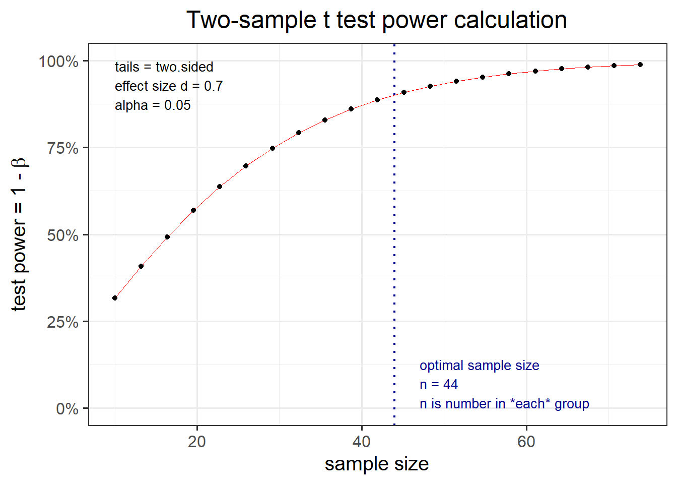
Let’s now slightly alter our perspective. Suppose that we already know that our survey will be limited by budget or time constraints and we can only afford to survey 40 individuals in total — that is, 20 in each group. Furthermore, we want to detect a difference in means of 0.60 standard deviations.
What’s the probability that you’ll be able to detect a difference between the population means that’s this large, given the constraints outlined?
res_t2 <- pwr.t.test(n = 20, d = 0.60, sig.level = 0.05,
                     type = "two.sample", alternative = "two.sided")
res_t2
##
## Two-sample t test power calculation
##
## n = 20
## d = 0.6
## sig.level = 0.05
## power = 0.4560341
## alternative = two.sided
##
## NOTE: n is number in *each* groupAffording only 20 participants per group, and only tolerating a 5% chance of a false discovery (i.e. rejecting the null when it is true), we would only be able to detect an effect of size 0.6 with a 45.6% chance, i.e. less than 50%. Similarly, you have a 50% chance of not finding the effect you’re looking for. The success rate of your test, given your survey constraints, is like flipping a coin! You might want to rethink this experiment, maybe try to improve the data collection or the design, otherwise you might end up wasting time.
If you wish to have different sample sizes in the two groups, n1 and n2, you should use the following R function
pwr.t2n.test(n1 = , n2 = , d = , sig.level = , power = , alternative = )Don’t be afraid of it, and try exploring it by varying its arguments!
B. Power for linear regression
In linear regression, the relevant function in R is
pwr.f2.test(u = , v = , f2 = , sig.level = , power = )where
u= numerator degrees of freedomv= denominator degrees of freedomf2= effect size
The formula for the effect size \(f^2\) is different depending on your goal.
Goal 1: Evaluating the impact of a set of predictors on an dependent variable.
Here you have one model, \[ y = \beta_0 + \beta_1 x_1 + \dots + \beta_k x_k + \epsilon \]
and you wish to find the minimum sample size required to answer the following test of hypothesis with a given power: \[ \begin{aligned} H_0 &: \beta_1 = \beta_2 = \dots = \beta_k = 0 \\ H_1 &: \text{At least one } \beta_i \neq 0 \end{aligned} \]
The appropriate formula for the effect size is: \[ f^2 = \frac{R^2}{1 - R^2} \]
And the numerator degrees of freedom are \(\texttt u = k\), the number of predictors in the model.
The denominator degrees of freedom returned by the function will give you: \[ \texttt v = n - (k + 1) = n - k - 1 \]
From which you can infer the sample size as \[ n = \texttt v + k + 1 \]
Goal 2: Evaluating the impact of extra predictors on an dependent variable, above and beyond other predictors.
In this case you would have a smaller model \(m\) with \(k\) predictors and a larger model \(M\) with \(K\) predictors: \[ \begin{aligned} m &: \quad y = \beta_0 + \beta_1 x_1 + \dots + \beta_{k} x_k + \epsilon \\ M &: \quad y = \beta_0 + \beta_1 x_1 + \dots + \beta_{k} x_k + \underbrace{\beta_{k + 1} x_{k+1} + \dots + \beta_{K} x_K}_{\text{extra predictors}} + \epsilon \end{aligned} \]
This case is when you wish to find the minimum sample size required to answer the following test of hypothesis: \[ \begin{aligned} H_0 &: \beta_{k+1} = \beta_{k+2} = \dots = \beta_K = 0 \\ H_1 &: \text{At least one of the above } \beta \neq 0 \end{aligned} \]
You need to use the R-squared from the larger model \(R^2_M\) and the R-squared from the smaller model \(R^2_m\). The appropriate formula for the effect size is: \[ f^2 = \frac{R^2_{M} - R^2_{m}}{1 - R^2_M} \]
Here, the numerator degrees of freedom are the extra predictors: \(\texttt u = K - k\).
The denominator degrees of freedom returned by the function will give you (here you use \(K\) the number of all predictors in the larger model): \[ \texttt v = n - (K + 1) = n - K - 1 \]
From which you can infer the sample size as \[ n = \texttt v + K + 1 \]
Recall the wellbeing/rurality study data? Let’s read them into R below:
library(tidyverse)
mwdata <- read_csv("https://uoepsy.github.io/data/wellbeing_rural.csv")
head(mwdata)
## # A tibble: 6 x 7
## age outdoor_time social_int routine wellbeing location steps_k
## <dbl> <dbl> <dbl> <dbl> <dbl> <chr> <dbl>
## 1 28 12 13 1 36 rural 21.6
## 2 56 5 15 1 41 rural 12.3
## 3 25 19 11 1 35 rural 49.8
## 4 60 25 15 0 35 rural NA
## 5 19 9 18 1 32 rural 48.1
## 6 34 18 13 1 34 rural 67.3Suppose you are interested in whether an individual’s routine and amount of social interactions per week impacts their wellbeing above and beyond their age, location and time spent outdoors.
Routine and amount of social interactions per week are 2 predictors, while age, location and time spent outdoors are 4 predictors (location needs 2 dummy variables!). So we are comparing a smaller model \(m\) with \(k = 4\) predictors to a larger model \(M\) with \(K = 4 + 2 = 6\) predictors.
Past experience suggests that age, location and time spent outdoors account for roughly 22% of the variability in wellbeing.
mdl_s <- lm(wellbeing ~ age + outdoor_time + location, data = mwdata)
summary(mdl_s)
##
## Call:
## lm(formula = wellbeing ~ age + outdoor_time + location, data = mwdata)
##
## Residuals:
## Min 1Q Median 3Q Max
## -12.2877 -3.0939 -0.2253 3.1799 18.9004
##
## Coefficients:
## Estimate Std. Error t value Pr(>|t|)
## (Intercept) 35.92645 1.51457 23.721 < 2e-16 ***
## age -0.01104 0.02281 -0.484 0.62899
## outdoor_time 0.17027 0.04794 3.551 0.00048 ***
## locationrural -4.47646 0.79657 -5.620 6.54e-08 ***
## locationsuburb -0.16077 0.96689 -0.166 0.86811
## ---
## Signif. codes: 0 '***' 0.001 '**' 0.01 '*' 0.05 '.' 0.1 ' ' 1
##
## Residual standard error: 4.777 on 195 degrees of freedom
## Multiple R-squared: 0.231, Adjusted R-squared: 0.2152
## F-statistic: 14.64 on 4 and 195 DF, p-value: 1.78e-10From a practical standpoint, it would be interesting if routine and social interactions per week accounted for at least 10% above this figure. Assuming a significance level of 0.05, how many subjects would be needed to identify such a contribution with 90% confidence?
The effect size here is: \[ f^2 = \frac{R^2_M - R^2_m}{1 - R^2_M} = \frac{0.32 - 0.22}{1 - 0.32} = 0.147 \]
Here,
sig.level = 0.05,power = 0.90,uis the number of extra predictors, so it will be \(K - k = 6 - 4 = 2\)- the effect size is the value computed before,
f2 = 0.147.
Entering this into the function yields the following:
pwr.f2.test(u = 2, f2 = 0.147, sig.level = 0.05, power = 0.90)##
## Multiple regression power calculation
##
## u = 2
## v = 86.15264
## f2 = 0.147
## sig.level = 0.05
## power = 0.9In multiple regression, the denominator degrees of freedom v equals \(n - K - 1\), where \(n\) is the sample size and \(K\) is the number of predictors in the larger model.
In this case, \(n - 6 - 1 = 87\), which means the required sample size is \(n = 87 + 6 + 1 = 94\).
Power curves
It might be also interesting to investigate the joint relationship between sample size and effect size.
First, we create a tibble containing a sequence seq of effect sizes to investigate, ranging for example from 0.1 to 0.9 in steps of 0.01: es = seq(.1, .9, .01).
Then, for each value in that sequence, we want to apply some computation. The computation is defined in
map_dbl(es,
        ~ pwr.f2.test(u = 2, f2 = .x, sig.level = 0.05, power = 0.9)$v)
This takes each element of es, one at a time, and then passes it to the computation specified afterwards, into the slot .x. Then, function pwr.f2.test is applied and we want to extract the value of v.
es_curve <- tibble(
    es = seq(.1, .9, .01),
    v = map_dbl(es,
                ~ pwr.f2.test(u = 2, f2 = .x, sig.level = 0.05, power = 0.9)$v)
)
es_curve
## # A tibble: 81 x 2
## es v
## <dbl> <dbl>
## 1 0.1 127.
## 2 0.11 115.
## 3 0.12 106.
## 4 0.13 97.4
## 5 0.14 90.5
## 6 0.15 84.4
## 7 0.16 79.2
## 8 0.17 74.5
## 9 0.18 70.4
## 10 0.19 66.7
## # ... with 71 more rowsNow, we want to compute \(n\) from v, using \(n - K - 1 = \texttt v\) so that \(n = \texttt v + K + 1\):
es_curve <- es_curve %>%
    mutate(n = v + 6 + 1)
es_curve
## # A tibble: 81 x 3
## es v n
## <dbl> <dbl> <dbl>
## 1 0.1 127. 134.
## 2 0.11 115. 122.
## 3 0.12 106. 113.
## 4 0.13 97.4 104.
## 5 0.14 90.5 97.5
## 6 0.15 84.4 91.4
## 7 0.16 79.2 86.2
## 8 0.17 74.5 81.5
## 9 0.18 70.4 77.4
## 10 0.19 66.7 73.7
## # ... with 71 more rowsLet’s see at the sample size required to find each effect size:
ggplot(es_curve, aes(n, es)) +
    geom_line() +
    labs(x = "Sample Size",
         y = "Effect Size",
         title = "Linear regression with power = 0.90 and alpha = 0.05")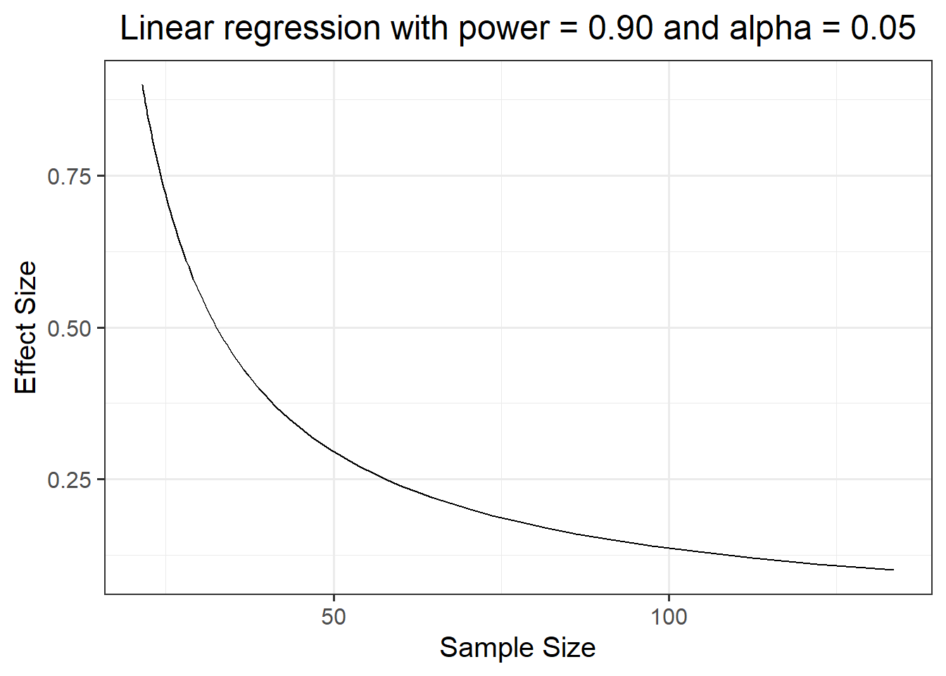
From the plot it looks like there is little gain in going beyond 100 observations.
Exercises
A sample of 200 individuals aged 18-75 years old was randomly allocated to either take a free-recall test after a 1-hour long roller-coaster session (group = 0) or a meditation session (group = 1). The data available from at the following link: https://uoepsy.github.io/data/recall_med_coast.csv
perc_recall: the percentage of correctly recalled itemsgroup: whether the individual was assigned to the roller-coaster (group = 0) or the meditation (group = 1) sessionage: the individual’s age
| perc_recall | group | age |
|---|---|---|
| 47.42891 | 0 | 52 |
| 61.44327 | 1 | 37 |
| 50.08974 | 0 | 46 |
| 56.44092 | 1 | 72 |
| 57.04785 | 1 | 46 |
| 46.11492 | 0 | 69 |
Using a significance level of 0.05, what sample size would you require to check whether any of the predictors (and interaction) influences recall scores with a 90% chance?
Because you do not know the effect size, assume Cohen’s guideline for linear regression and, to be on the safe side, consider the “Small” value.
Using the same \(\alpha\) and power, what would be the sample size if you assumed effect size to be medium?
Using the same \(\alpha\) and power, what would be the sample size if you assumed effect size to be large?
Read the data into R and make sure that all variables are correctly encoded.
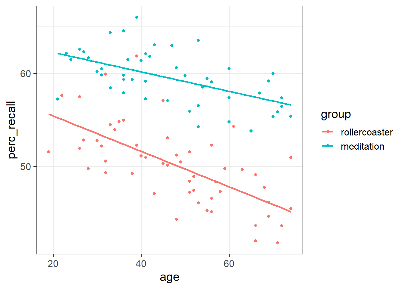
Display a scatterplot investigating the relationship between recall and age by group.
Using geom_smooth(), also display the regression line for each group.
Is there any evidence of an interaction between age and group?
Fit a model with just age as a predictor of recall. What is the R-squared?
Imagine you found the R-squared that you computed above in a paper, and you are using that to base your next study.
A researcher believes that the inclusion of group and its interaction with age should explain an extra 50% of the variation in recall scores.
Using a significance level of 5%, what sample size should you use for your next data collection in order to discover that effect with a power of 0.9?
Suppose that the addition of group and its interaction with age, to the R-squared from the literature, was thought to explain only 5% more of the variability in recall scores.
Using a significance level of 5%, what sample size should you use for your next data collection in order to discover that effect with a power of 0.9?
Cohen, J. (1988) Statistical Power Analysis for the Behavioral Sciences, 2nd ed. Hillsdale, NJ: Lawrence Erlbaum.↩︎
Cohen J. (1992) A power primer, Psychological Bulletin, 112(1): 155–159. PDF available via the University of Edinburgh library at this link.↩︎