Coding Factors

LEARNING OBJECTIVES

1. Understand how to specify dummy and effects coding
2. Understand how to specify contracts to test specific effects

Research question

Do you think the type of background music playing in a restaurant influences the amount of money that diners spend on their meal?

Data: RestaurantSpending.csv

Download link

Download the data here

Description

A group of researchers wanted to test the claims reported in (North, Shilcock, and Hargreaves 2003) on whether the type of background music playing in a restaurant influences the average amount of money spent by diners on their meal.

The group researchers got in touch with a restaurant and asked to alternate silence, popular music, and classical music on successive nights over 18 days. On those nights they recorded the mean spend per head for each table.

The following variables were collected:

• id: Identifier for each diner
• type: type of music played (“Classical Music,” “Pop Music,” “No Music”)
• amount: restaurant spending per person (in pounds - £)

Preview

The top six rows of the data are as follows:

id	type	amount
1	No Music	23.15
2	Pop Music	20.59
3	Pop Music	19.18
4	Pop Music	16.7
5	Classical Music	25.91
6	Pop Music	19.28

Data Exploration: Descriptives

Question 1

1. Load the tidyverse package.
2. Read the restaurant spending data into R using the function read_csv() and name the data rest_spend.
3. Check for the correct coding of all variables (i.e., categorical variables should be factors and numeric variables should be numeric).

Solution

Load the tidyverse library:

library(tidyverse)

Read the data into R:

rest_spend <- read_csv('https://uoepsy.github.io/data/RestaurantSpending.csv')

Check if the data were read into R correctly by examining the top six rows:

head(rest_spend)

## # A tibble: 6 x 3
##      id type            amount
##   <dbl> <chr>            <dbl>
## 1     1 No Music          23.1
## 2     2 Pop Music         20.6
## 3     3 Pop Music         19.2
## 4     4 Pop Music         16.7
## 5     5 Classical Music   25.9
## 6     6 Pop Music         19.3

Music type is a categorical variable but it is encoded as a character (<chr>) variable rather than a factor (<fctr>). Let’s fix this:

# We could do this the standard way
rest_spend$type <- as.factor(rest_spend$type)

# Or the tidyverse way
rest_spend <- rest_spend %>%
  mutate(type = as.factor(type))

And check again:

head(rest_spend)

## # A tibble: 6 x 3
##      id type            amount
##   <dbl> <fct>            <dbl>
## 1     1 No Music          23.1
## 2     2 Pop Music         20.6
## 3     3 Pop Music         19.2
## 4     4 Pop Music         16.7
## 5     5 Classical Music   25.9
## 6     6 Pop Music         19.3

Question 2

Produce a boxplot displaying the relationship between restaurant spending and music type, and comment on any visually observed differences among the sample means of the three background music types.

Solution

ggplot(data = rest_spend, aes(x = type, y = amount)) +
  geom_boxplot() +
  labs(x = 'Background music type', y = 'Restaurant spending (in GBP)')

From the boxplots, it seems that customers without background music or pop music had a similar average restaurant spending.

Furthermore, the average restaurant spending seems to be higher for those who had a classical music background compared to the customers either without music or with a pop music background.

Question 3

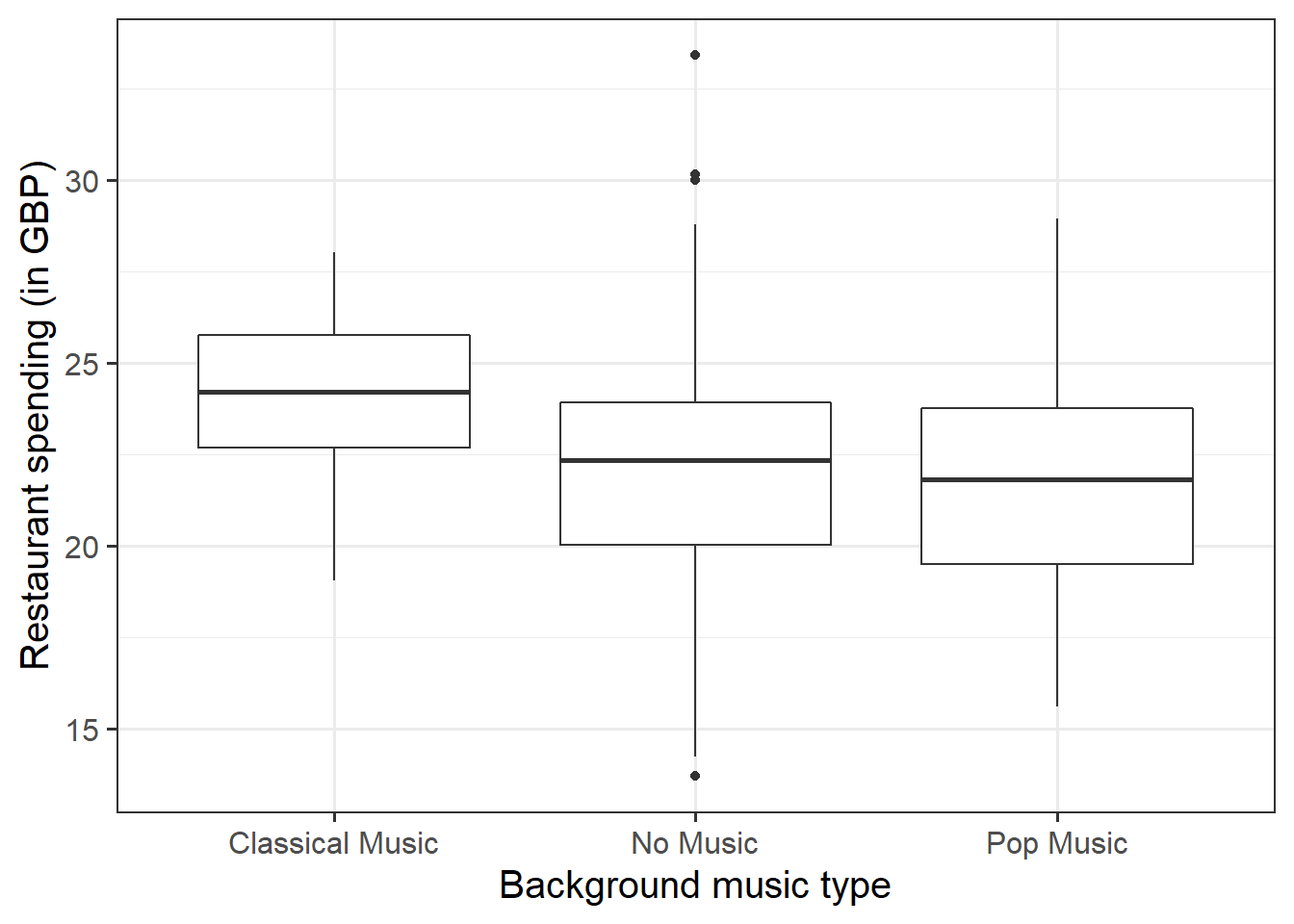
For the restaurant spending data, what is the number of groups (\(g\)) and the numbers of observations per group (\(n\))? What was the average spending and standard deviation of each group?

Solution

rest_spend %>%
  group_by(type) %>%
  summarise(n = n(), 
            M = mean(amount), 
            SD = sd(amount))

## # A tibble: 3 x 4
##   type                n     M    SD
##   <fct>           <int> <dbl> <dbl>
## 1 Classical Music   120  24.2  1.89
## 2 No Music          120  22.1  3.44
## 3 Pop Music         120  21.9  2.97

There are three groups, one for each music type: “Classical Music,” “No Music,” “Pop Music.” Hence, \(g = 3\). There are 120 observations for each group, i.e. \(n = 120\).

Levels of Variable & Side Constraints

Levels of variable

R by default orders the levels of a categorical variable in alphabetical order:

levels(rest_spend$type)

## [1] "Classical Music" "No Music"        "Pop Music"

If we follow the same approach and order the groups by alphabetical ordering, we can represent the data as follows:

Population Name	Population ID	Sample observations	Population mean
Classical Music	1	\(y_{1,1}, y_{1,2}, ..., y_{1,n}\)	\(\mu_{1}\)
No Music	2	\(y_{2,1}, y_{2,2}, ..., y_{2,n}\)	\(\mu_{2}\)
Pop Music	3	\(y_{3,1}, y_{3,2}, ..., y_{3,n}\)	\(\mu_{3}\)

Sum to zero constraint - effects coding

Under the constraint \(\beta_1 + \beta_2 + \beta_3 = 0\), the model coefficients are interpreted as follows:

• \(\beta_0 = \mu\) is interpreted as the overall or global mean — that is, the population mean when all the groups are combined;
• \(\beta_i = \mu_i - \mu\) is interpreted as the effect of group \(i\) — that is, the difference between the population mean for group \(i\), \(\mu_i\), and the global population mean, \(\mu\).

We can fit the linear regression model:

\[ y = b_0 + b_1 \ \text{EffectLevel1} + b_2 \ \text{EffectLevel2} + \epsilon \]

where

\[ \text{EffectLevel1} = \begin{cases} 1 & \text{if observation is from category 1} \\ 0 & \text{if observation is from category 2} \\ -1 & \text{otherwise} \end{cases} \\ \text{EffectLevel2} = \begin{cases} 0 & \text{if observation is from category 1} \\ 1 & \text{if observation is from category 2} \\ -1 & \text{otherwise} \end{cases} \]

Schematically,

\[ \begin{matrix} \textbf{Level} & \textbf{EffectLevel1} & \textbf{EffectLevel2} \\ \hline \text{Classical Music} & 1 & 0 \\ \text{No Music} & 0 & 1 \\ \text{Pop Music} & -1 & -1 \end{matrix} \]

In R this is simply done by saying:

contrasts(rest_spend$type) <- "contr.sum"
mdl_sum <- lm(amount ~ type, data = rest_spend)
coef(mdl_sum)

## (Intercept)       type1       type2 
##  22.7381560   1.4359846  -0.5967688

where type is a factor. In such case R will automatically create the two variables EffectLevel1 and EffectLevel2 for you!

The summary(mdl) will return 3 estimated coefficients:

• \(b_0 = 22.74\) is estimated overall mean
• \(b_1 = 1.44\) is the effect of Classical Music
• \(b_2 = -0.6\) is the effect of No Music
• NOTE: The effect of Pop Music is not shown by summary as it is found via the side-constraint as \(b_3 = -(b_1 + b_2) = -0.84\)!

Reference group constraint - dummy coding

Under the constraint \(\beta_1 = 0\), meaning that the first factor level is the reference group,

• \(\beta_0\) is interpreted as \(\mu_1\), the mean response for the reference group (group 1);
• \(\beta_i\) is interpreted as the difference between the mean response for group \(i\) and the reference group.

We can fit the linear regression model:

\[ y = b_0 + b_1 \ \text{IsTypeNoMusic} + b_2 \ \text{IsTypePopMusic} +\epsilon \]

where

\[ \text{IsTypeNoMusic} = \begin{cases} 1 & \text{if observation is from the No Music category} \\ 0 & \text{otherwise} \end{cases} \\ \text{IsTypePopMusic} = \begin{cases} 1 & \text{if observation is from the Pop Music category} \\ 0 & \text{otherwise} \end{cases} \]

Schematically,

\[ \begin{matrix} \textbf{Level} & \textbf{IsTypeNoMusic} & \textbf{IsTypePopMusic} \\ \hline \text{Classical Music} & 0 & 0 \\ \text{No Music} & 1 & 0 \\ \text{Pop Music} & 0 & 1 \end{matrix} \]

In R this is simply done by saying:

contrasts(rest_spend$type) <- "contr.treatment"
mdl_trt <- lm(amount ~ type, data = rest_spend)
coef(mdl_trt)

##   (Intercept)  typeNo Music typePop Music 
##     24.174141     -2.032753     -2.275200

where type is a factor. In such case R will automatically create the two dummy variables IsTypeNoMusic and IsTypePopMusic for you!

The summary(mdl) will return 3 estimated coefficients:

• \(b_0 = 24.17\) is the mean of the base level (level 1)
• \(b_1 = -2.03\) is the effect of No Music
• \(b_2 = -2.28\) is the effect of Pop Music
• NOTE: The effect of Classical Music is not shown as it is equal to zero by the constraint!

Side Contraints

Possible side-constraints on the parameters are:

Name	Constraint	Meaning of \(\beta_0\)	R
Sum to zero (Effects Coding)	\(\beta_1 + \beta_2 + \beta_3 = 0\)	\(\beta_0 = \mu\)	contr.sum
Reference group (Dummy Coding)	\(\beta_1 = 0\)	\(\beta_0 = \mu_1\)	contr.treatment

IMPORTANT

• By default R uses the reference group constraint

• If your factor has \(g\) levels, your regression model will have \(g-1\) dummy variables (R creates them for you)

ANOVA F-test

Since R uses the reference group constraint, in this section and the next one, we will not specify any side-constraints, meaning that \(\beta_1 = 0\).

Question 4

Fit a linear model to the data, having amount as response variable and the factor type as predictor. Call the fitted model mdl_rg (for reference group constraint)

Identify the relevant pieces of information from the commands anova(mdl_rg) and summary(mdl_rg) that can be used to conduct an ANOVA F-test against the null hypothesis that all population means are equal.

Interpret the F-test results in the context of the ANOVA null hypothesis.

Solution

mdl_rg <- lm(amount ~ type, data = rest_spend)
mdl_rg

## 
## Call:
## lm(formula = amount ~ type, data = rest_spend)
## 
## Coefficients:
##   (Intercept)   typeNo Music  typePop Music  
##        24.174         -2.033         -2.275

summary(mdl_rg)

## 
## Call:
## lm(formula = amount ~ type, data = rest_spend)
## 
## Residuals:
##    Min     1Q Median     3Q    Max 
## -8.433 -1.886  0.127  1.755 11.285 
## 
## Coefficients:
##               Estimate Std. Error t value Pr(>|t|)    
## (Intercept)    24.1741     0.2593  93.211  < 2e-16 ***
## typeNo Music   -2.0328     0.3668  -5.542 5.81e-08 ***
## typePop Music  -2.2752     0.3668  -6.203 1.53e-09 ***
## ---
## Signif. codes:  0 '***' 0.001 '**' 0.01 '*' 0.05 '.' 0.1 ' ' 1
## 
## Residual standard error: 2.841 on 357 degrees of freedom
## Multiple R-squared:  0.1151, Adjusted R-squared:  0.1101 
## F-statistic: 23.21 on 2 and 357 DF,  p-value: 3.335e-10

anova(mdl_rg)

## Analysis of Variance Table
## 
## Response: amount
##            Df Sum Sq Mean Sq F value    Pr(>F)    
## type        2  374.7 187.348  23.211 3.335e-10 ***
## Residuals 357 2881.5   8.071                      
## ---
## Signif. codes:  0 '***' 0.001 '**' 0.01 '*' 0.05 '.' 0.1 ' ' 1

The model summary returns the F-test of model utility which, in this case, corresponds to the ANOVA F-test against the null hypothesis of equal population means.

The relevant line from summary() is:

F-statistic: 23.21 on 2 and 357 DF,  p-value: 3.335e-10

The relevant parts from anova() are:

• F value of 23.211
• The Df column giving 2 and 357 degrees of freedom
• The p-value of the test, reported under Pr(>F) as 3.335e-10 ***.

We can write this up as follows:

We performed an analysis of variance against the null hypothesis of equal population mean spending across three types of background music, \(F(2, 357) = 23.21\), \(p < .001\).

The large observed F statistic leads to a very small p-value, meaning that such a large observed variability among the mean restaurant spending across the different music types, compared to the variability in the residuals, is very unlikely to happen by chance alone if the population means where all the same.

For this reason, at the 5% significance level we reject the null hypothesis as there is strong evidence that at least two population means differ.

Reference group (dummy) constraint

Question 5

Examine and investigate the meaning of the coefficients in the output of summary(mdl_rg). Next, obtain the estimated (or predicted) group means for the “Classical Music,” “No Music,” and “Pop Music” groups by using the predict(mdl_rg, newdata = ...) function.

Solution

Let’s recall the model summary:

summary(mdl_rg)

## 
## Call:
## lm(formula = amount ~ type, data = rest_spend)
## 
## Residuals:
##    Min     1Q Median     3Q    Max 
## -8.433 -1.886  0.127  1.755 11.285 
## 
## Coefficients:
##               Estimate Std. Error t value Pr(>|t|)    
## (Intercept)    24.1741     0.2593  93.211  < 2e-16 ***
## typeNo Music   -2.0328     0.3668  -5.542 5.81e-08 ***
## typePop Music  -2.2752     0.3668  -6.203 1.53e-09 ***
## ---
## Signif. codes:  0 '***' 0.001 '**' 0.01 '*' 0.05 '.' 0.1 ' ' 1
## 
## Residual standard error: 2.841 on 357 degrees of freedom
## Multiple R-squared:  0.1151, Adjusted R-squared:  0.1101 
## F-statistic: 23.21 on 2 and 357 DF,  p-value: 3.335e-10

The interpretation is as follows

Coefficient	Estimate	Corresponds to
(Intercept)	24.1741	\(\hat \beta_0 = \hat \mu_1\)
typeNo Music	-2.0328	\(\hat \beta_2 = \hat \mu_2 - \hat \beta_0 = \hat \mu_2 - \hat \mu_1\)
typePop Music	-2.2752	\(\hat \beta_3 = \hat \mu_3 - \hat \beta_0 = \hat \mu_3 - \hat \mu_1\)

The estimate corresponding to (Intercept) contains \(\hat \beta_0 = \hat \mu_1 = 24.17\). The estimated average spending for those having a classical music background is approximately £24.2.

The next estimate corresponds to typeNo Music and is \(\hat \beta_2 = -2.033\). The difference in mean spending between No Music and Classical Music is estimated to be \(-2.033\). In other words, people with a silent background seem to spend approximately £2 less than those having a classical music background.

The estimate corresponding to typePop Music is \(\hat \beta_3 = -2.275\). This is the estimated difference in mean spending between Pop Music and Classical Music. People with a pop music background seem to spend approximately £2.3 less than those with a classical music background.

Hence, for all levels except the reference group we see differences to the reference group while the estimate of the reference level can be found next to (Intercept).

It is also important to notice how the coefficients names are written. They are a combination of factor name and level name, such as typeNo Music. The only coefficient that is missing is typeClassical Music, the one corresponding to the reference category Classical Music.

To use preditct, you first need to define a data frame with a column having the same name as the factor in the fitted model. Then, specify all the groups (= levels) for which you would like the predicted mean.

query_groups <- tibble(type = c("Classical Music", "No Music", "Pop Music"))
query_groups

## # A tibble: 3 x 1
##   type           
##   <chr>          
## 1 Classical Music
## 2 No Music       
## 3 Pop Music

Pass the data frame to the predict function using the newdata = argument. The predict function will match the column named type with the predictor called type in the fitted model mdl_rg.

predict(mdl_rg, newdata = query_groups)

##        1        2        3 
## 24.17414 22.14139 21.89894

Or:

query_groups %>%
  mutate(pred = predict(mdl_rg, newdata = .))

## # A tibble: 3 x 2
##   type             pred
##   <chr>           <dbl>
## 1 Classical Music  24.2
## 2 No Music         22.1
## 3 Pop Music        21.9

Hence,

• \(\hat \mu_\text{Classical Music} = \hat \mu_1 = 24.17\)
• \(\hat \mu_\text{No Music} = \hat \mu_2 = 22.14\)
• \(\hat \mu_\text{Pop Music} = \hat \mu_3 = 21.90\)

Question 6

It actually makes more sense to have “No Music” as reference group.

Open the help page of the function fct_relevel(), and look at the examples.

Within the rest_sped data, reorder the levels of the factor type so that your reference group is “No Music.”

NOTE

Because you reordered the levels, now

• \(\mu_1\) = mean of no music group
• \(\mu_2\) = mean of classical music group
• \(\mu_3\) = mean of pop music group

Solution

Check the help page:

?fct_relevel

Select “No Music” to be the first level:

rest_spend$type <- fct_relevel(rest_spend$type, "No Music")

Check that the factor levels are now in the correct order:

levels(rest_spend$type)

## [1] "No Music"        "Classical Music" "Pop Music"

Question 7

Refit the linear model, and inspect the model summary once more.

Do you notice any change in the estimated coefficients? Do you notice any change in the F-test for model utility?

Solution

mdl_rg <- lm(amount ~ type, data = rest_spend)
summary(mdl_rg)

## 
## Call:
## lm(formula = amount ~ type, data = rest_spend)
## 
## Residuals:
##    Min     1Q Median     3Q    Max 
## -8.433 -1.886  0.127  1.755 11.285 
## 
## Coefficients:
##                     Estimate Std. Error t value Pr(>|t|)    
## (Intercept)          22.1414     0.2593  85.373  < 2e-16 ***
## typeClassical Music   2.0328     0.3668   5.542 5.81e-08 ***
## typePop Music        -0.2424     0.3668  -0.661    0.509    
## ---
## Signif. codes:  0 '***' 0.001 '**' 0.01 '*' 0.05 '.' 0.1 ' ' 1
## 
## Residual standard error: 2.841 on 357 degrees of freedom
## Multiple R-squared:  0.1151, Adjusted R-squared:  0.1101 
## F-statistic: 23.21 on 2 and 357 DF,  p-value: 3.335e-10

The displayed coefficients have changed as now the (Intercept) represents the new reference group, which is “No Music.”

However, by checking the calculations, this model is equivalent to the previous one as the predicted group means are the same.

• Predicted mean of “No Music” \(\hat \mu_\text{No Music}\) = 22.1414
• Predicted mean of “Classical Music” \(\hat \mu_\text{Classical Music}\) = 22.1414 + 2.0328 = 24.1742
• Predicted mean of “Pop Music” = \(\hat \mu_\text{Pop Music}\) = 22.1414 - 0.2424 = 21.899

The predict function returns the same output:

query_groups <- tibble(type = levels(rest_spend$type))
query_groups

## # A tibble: 3 x 1
##   type           
##   <chr>          
## 1 No Music       
## 2 Classical Music
## 3 Pop Music

query_groups %>% 
  mutate(pred = predict(mdl_rg, newdata = .))

## # A tibble: 3 x 2
##   type             pred
##   <chr>           <dbl>
## 1 No Music         22.1
## 2 Classical Music  24.2
## 3 Pop Music        21.9

Sum-to-zero (effects) constraint

Let’s now change the side-constraint from the R default (the reference group or contr.treatment constraint) to the sum-to-zero constraint using contr.sum.

Recall that under this constraint the interpretation of the coefficients becomes:

• \(\beta_0\) represents the global mean
• \(\beta_i\) the effect due to group \(i\) — that is, the mean response in group \(i\) minus the global mean

Question 8

Set the sum to zero constraint for the factor type of background music.

Fit again the linear model using amount as response variable and type as predictor. Call the fitted model using the sum to zero constraint mdl_stz (for sum to zero).

Examine the output of the summary(mdl_stz) function:

• Do the displayed coefficients change? What do they represent now?
• Do the predicted group means change?
• Is the model utility F-test still the same? Why do you think it’s the case?

Solution

Set the sum to zero contrast to the type factor:

contrasts(rest_spend$type) <- "contr.sum"

Re-fit the model and inspect the summary output:

mdl_stz <- lm(amount ~ type, data = rest_spend)
summary(mdl_stz)

## 
## Call:
## lm(formula = amount ~ type, data = rest_spend)
## 
## Residuals:
##    Min     1Q Median     3Q    Max 
## -8.433 -1.886  0.127  1.755 11.285 
## 
## Coefficients:
##             Estimate Std. Error t value Pr(>|t|)    
## (Intercept)  22.7382     0.1497 151.856  < 2e-16 ***
## type1        -0.5968     0.2118  -2.818   0.0051 ** 
## type2         1.4360     0.2118   6.781 4.95e-11 ***
## ---
## Signif. codes:  0 '***' 0.001 '**' 0.01 '*' 0.05 '.' 0.1 ' ' 1
## 
## Residual standard error: 2.841 on 357 degrees of freedom
## Multiple R-squared:  0.1151, Adjusted R-squared:  0.1101 
## F-statistic: 23.21 on 2 and 357 DF,  p-value: 3.335e-10

With the new side-constraint, we get different values for the model coefficients because the meaning of the parameters has changed. If we closely inspect the output, we can also notice that a slightly different naming has been used.

Instead of factor name and level name (such as typeNo Music), we get factor name and level number (e.g. type1). Here, type1 simply means the first level of the factor type, while type2 means the second level of the factor type.

levels(rest_spend$type)

## [1] "No Music"        "Classical Music" "Pop Music"

The first level is “No Music,” while the second level is “Classical Music.”

• The estimate for (Intercept) is now the global mean of the data.
• The estimate for type1 is now the difference of the first group (“No Music”) to the global mean
• The estimate for type2 is now the difference of the second group (“Classical Music”) to the global mean

The estimate for type3, representing the difference of “Pop Music” to the global mean is not shown. Because of the side-constraint, we know it must be \(\beta_3 = - (\beta_1 + \beta_2) = - (-0.5968 + 1.4360) = -0.8392\).

Underneath we see the group effects that need to be added to the global mean to obtain the predicted group means.

Compute the predicted group means:

query_groups %>%
  mutate(pred = predict(mdl_stz, newdata = .))

## # A tibble: 3 x 2
##   type             pred
##   <chr>           <dbl>
## 1 No Music         22.1
## 2 Classical Music  24.2
## 3 Pop Music        21.9

We notice that we get the same predicted group means independently of the side-constraint.

The predicted means do not depend on the side-constraint that we apply. However, the side-constraint influences the meaning of the parameters in the model.

In R, we can switch back to the default reference group constraint by either of these

# Option 1
contrasts(rest_spend$type) <- NULL
# Option 2
contrasts(rest_spend$type) <- "contr.treatment"

Contrasts

We have seen that the F-test (and incremental F-test using anova()) provide overall tests of whether there are differences in the group means. When we use dummy (reference) coding, this could be a difference between one group and the reference group. When we use effects (sum-to-zero) coding, this could be a difference between one group and the grand mean. In some cases the investigators will have pre-planned comparisons they would like to make, and it is this we will look at next. To do so, we will use a package called emmeans.

Contrasts represent a wide range of hypotheses about the population means that can be tested using the fitted model.

However, they need to match the following general form. A contrast only allows us to test hypotheses that can be written as a linear combination of the population means with coefficients summing to zero: \[ H_0 : c_1 \mu_1 + c_2 \mu_2 + c_3 \mu_3 = 0 \qquad \text{with} \qquad c_1 + c_2 + c_3 = 0 \]

#install.packages("emmeans") remember that you only install packages once, and you should do so in the console, not your .Rmd script
library(emmeans)

Question 9

We were interested in the following comparisons:

• Whether having some kind of background music, rather than no music, makes a difference in mean restaurant spending
• Whether there is any difference in mean restaurant spending between those with no background music and those with pop music

These are planned comparisons and can be translated to the following research hypotheses: \[ \begin{aligned} 1. \quad H_0 &: \mu_\text{No Music} = \frac{1}{2} (\mu_\text{Classical Music} + \mu_\text{Pop Music}) \\ 2. \quad H_0 &: \mu_\text{No Music} = \mu_\text{Pop Music} \end{aligned} \]

First of all check the levels of the factor type, as the contrast coefficients need to match the order of the levels:

levels(rest_spend$type)

## [1] "No Music"        "Classical Music" "Pop Music"

We specify the hypotheses by first giving each a name, and then specify the coefficients of the comparisons:

comp <- list("No Music - Some Music" = c(1, -1/2, -1/2),
             "No Music - Pop Music" = c(1, 0, -1))

Use the emmeans() function to obtain the estimated treatment means and uncertainties for your factor:

emm <- emmeans(mdl_stz, ~ type)
emm

##  type            emmean    SE  df lower.CL upper.CL
##  No Music          22.1 0.259 357     21.6     22.7
##  Classical Music   24.2 0.259 357     23.7     24.7
##  Pop Music         21.9 0.259 357     21.4     22.4
## 
## Confidence level used: 0.95

Next, we run the contrast analysis. To do so, we use the contrast() function:

comp_res <- contrast(emm, method = comp)
comp_res

##  contrast              estimate    SE  df t.ratio p.value
##  No Music - Some Music   -0.895 0.318 357  -2.818  0.0051
##  No Music - Pop Music     0.242 0.367 357   0.661  0.5090

Finally, we can ask for 95% confidence intervals:

confint(comp_res)

##  contrast              estimate    SE  df lower.CL upper.CL
##  No Music - Some Music   -0.895 0.318 357   -1.520   -0.270
##  No Music - Pop Music     0.242 0.367 357   -0.479    0.964
## 
## Confidence level used: 0.95

Interpret the result of the contrast analysis.

• What do the p-values tell us?
• Interpret the confidence intervals in the context of the study.

Solution

The hypothesis test for the first contrast could be reported as follows:

We performed a test against \(H_0: \mu_1 - \frac{1}{2}(\mu_2 + \mu_3) = 0\), resulting in \(t(357) = -2.818, p = .005\), two-sided. At the 5% significance level, there is strong evidence that the mean spending for those with no music is different than the mean spending for those with some of background music.

The 95% confidence interval for \(\mu_1 - \frac{1}{2}(\mu_2 + \mu_3)\) is given by \([-1.520, -0.270]\).

The corresponding confidence interval could be written up as:

We are 95% confident that diners with no background music will spend, on average, between £1.52 and £0.27 pounds less than those with some background music.

The hypothesis test for the second contrast could be reported as follows:

We performed a test against \(H_0: \mu_1 - \mu_3 = 0\), resulting in \(t(357) = 0.661, p = .509\), two-sided. At the 5% significance level, there is not sufficient evidence to reject the null hypothesis that the mean spending for those with no music is the same as the mean spending for those with pop music.

The 95% confidence interval for \(\mu_1 - \mu_3\) is given by \([-0.479, 0.964]\).

Because we have established that there isn’t a significant difference between the mean spending for those with no music and those with pop music, we will not interpret the confidence interval.

A final situation is where an investigator has no predetermined ideas at all where differences may lie, and they may wish to explore the data. We will discuss methods for such analyses in future weeks.

References

North, A., A. Shilcock, and D. Hargreaves. 2003. “The Effect of Musical Style on Restaurant Customers’ Spending.” Environment and Behavior 35: 712–18.