Assumptions & Diagnostics

In this lab, you will be provided with a comprehensive overview of linear regression assumptions and diagnostics. Therefore, whilst the lab might be appear rather lengthy, it will serve as a handy reference for you to use in the future and refer back to when needed.

LEARNING OBJECTIVES

1. Be able to state the assumptions underlying a linear model.
2. Specify the assumptions underlying a linear model with multiple predictors.
3. Assess if a fitted model satisfies the assumptions of your model.
4. Assess the effect of influential cases on linear model coefficients and overall model evaluations.

Linear Model Assumptions

In the previous labs, we have fitted a number of regression models, including some with multiple predictors. In each case, we first specified the model, then visually explored the marginal distributions and relationships of variables which would be used in the analysis. Finally, we fit the model, and began to examine the fit by studying what the various parameter estimates represented, and the spread of the residuals (the parts of the output inside the red boxes in Figure 1)

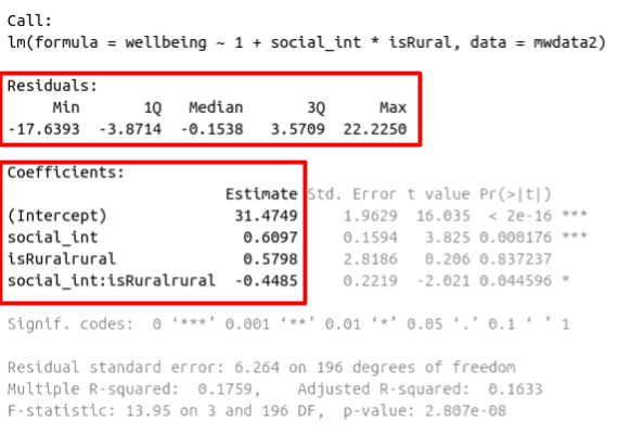
Figure 1: Multiple regression output in R, summary.lm(). Residuals and Coefficients highlighted

But before we draw inferences using our model estimates or use our model to make predictions, we need to be satisfied that our model meets a specific set of assumptions. If these assumptions are not satisfied, the results will not hold.

All of the estimates, intervals and hypothesis tests (see Figure 2) resulting from a regression analysis assume a certain set of conditions have been met. Meeting these conditions is what allows us to generalise our findings beyond our sample (i.e., to the population).

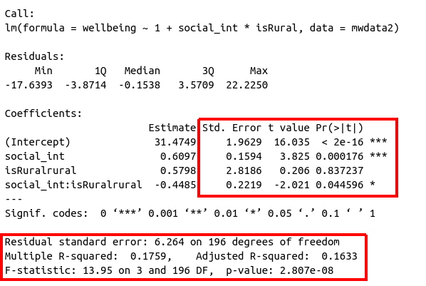
Figure 2: Multiple regression output in R, summary.lm(). Hypothesis tests highlighted

You can remember the four assumptions by memorising the acronym LINE:

• L - Linearity
• I - Independence
• N - Normality
• E - Equal variance

If at least one of these assumptions does not hold, say N - Normality, you might be reporting a LIE. Recall the assumptions of the linear model:

• Linearity: The relationship between \(y\) and \(x\) is linear.
• Independence of errors: The error terms should be independent from one another.
• Normality: The errors \(\epsilon\) are normally distributed in the population.
• Equal variances (“Homoscedasticity”): The variability of the errors \(\epsilon\) is constant across \(x\).

Because we don’t have the data about the entire population, we check the assumptions on the errors by looking at their sample counterpart: the residuals from the fitted model = observed values - fitted values = \(y_i - \hat y_i\).
The residuals \(\hat \epsilon_i\) are the sample realisation of the actual, but unknown, true errors \(\epsilon_i\) for the entire population. Because these same assumptions hold for a regression model with multiple predictors, we can assess them in a similar way. However, there are a number of important considerations.

In this lab, we will check the assumptions of two models - one simple linear model, and one with multiple predictors, and assess whether these models meet the assumptions outlined above. We will be working with two different datasets that you have used in previous labs: riverview and wellbeing.

Guided exercises

Open a new RMarkdown document. Copy the code below to load in the tidyverse packages, read in the riverview.csv and wellbeing.csv datasets and fit the following two models:

\[ \begin{aligned} M1&: \quad \text{Income} = \beta_0 + \beta_1 \cdot \text{Education} + \epsilon \\ M2&: \quad \text{Wellbeing} = \beta_0 + \beta_1 \cdot \text{Outdoor Time} + \beta_2 \cdot \text{Social Interactions} + \epsilon \end{aligned} \]

library(tidyverse) 

# read in the riverview data
rvdata <- read_csv(file = "https://uoepsy.github.io/data/riverview.csv")

# read in the wellbeing data
wbdata <-  read_csv(file = "https://uoepsy.github.io/data/wellbeing.csv")

# fit the linear models: 
rv_mdl1 <- lm(income ~ 1 + education, data = rvdata) #riverview model

wb_mdl1 <- lm(wellbeing ~ outdoor_time + social_int, data = wbdata) #wellbeing model

Note: We have have forgone writing the 1 in lm(y ~ 1 + x.... The 1 just tells R that we want to estimate the Intercept, and it will do this by default even if we leave it out.

Linearity

Simple Linear Regression

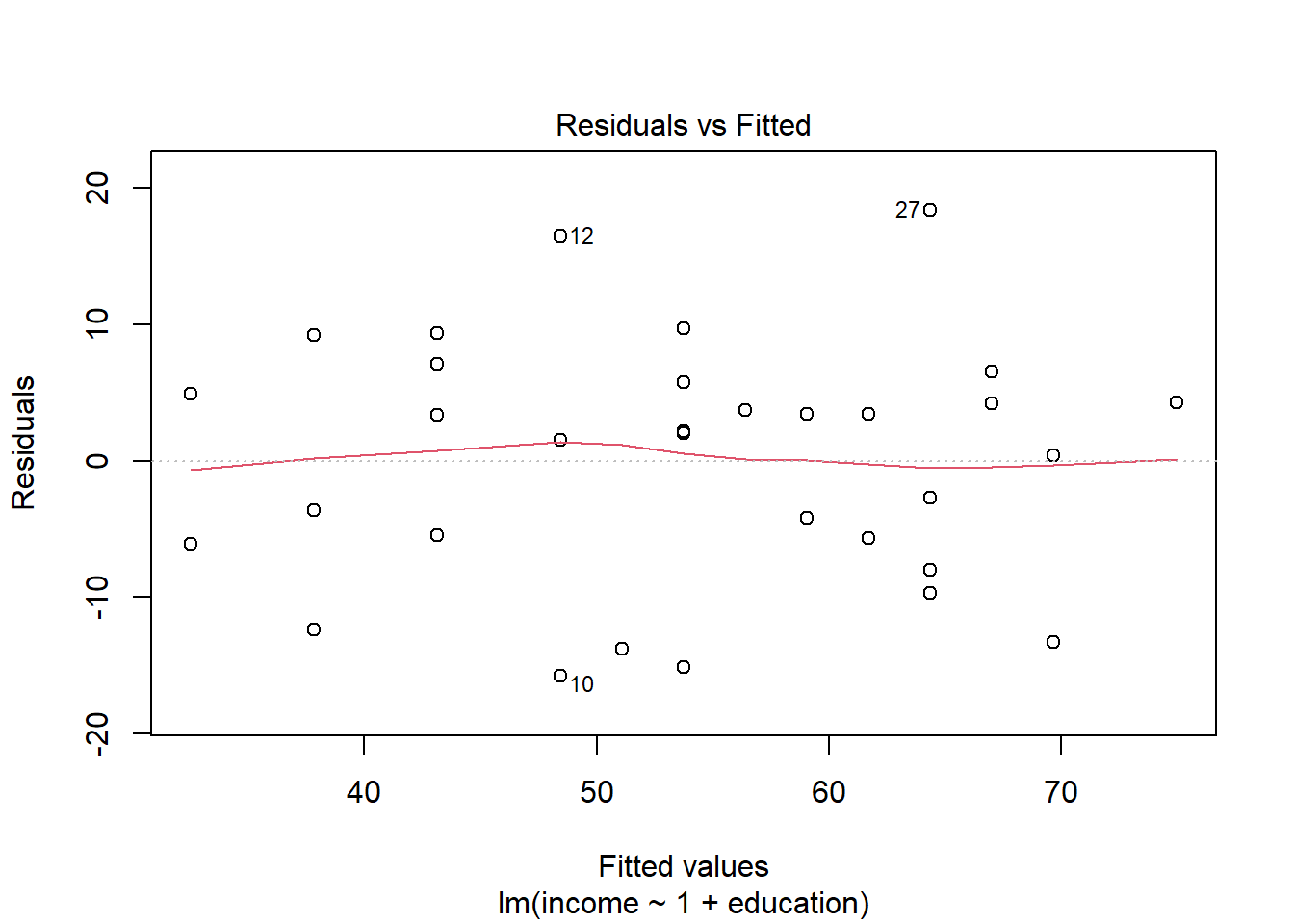
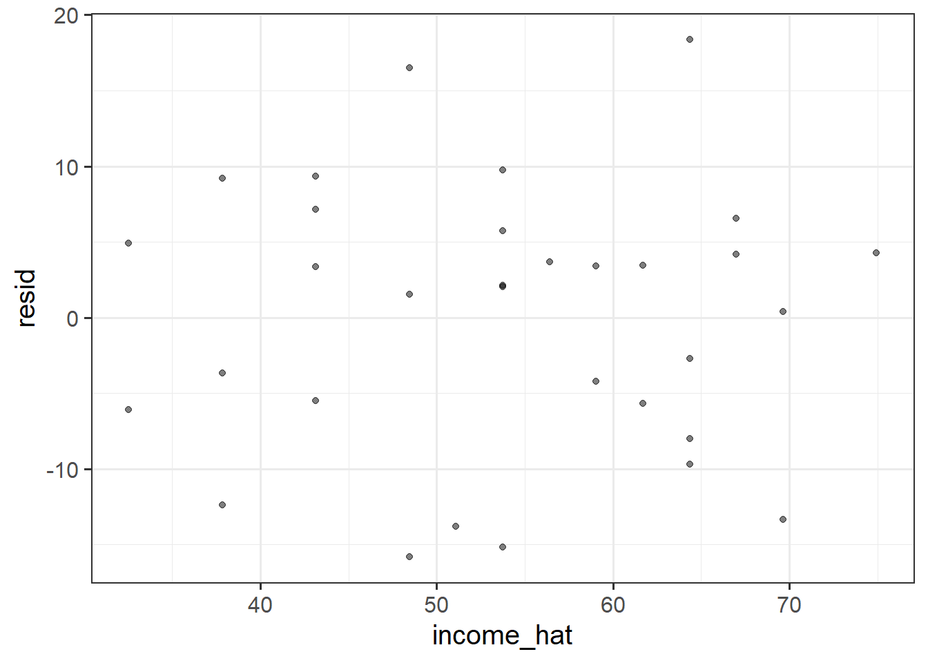
In simple linear regression (SLR) with only one explanatory variable, we could assess linearity through a simple scatterplot of the outcome variable against the explanatory. This would allow us to check if the errors have a mean of zero. If this assumption was met, the residuals would appear to be randomly scattered around zero.
The rationale for this is that, once you remove from the data the linear trend, what’s left over in the residuals should not have any trend, i.e. have a mean of zero.

Multiple Regression

In multiple regression, however, it becomes more necessary to rely on diagnostic plots of the model residuals. This is because we need to know whether the relations are linear between the outcome and each predictor after accounting for the other predictors in the model.

In order to assess this, we use partial-residual plots (also known as ‘component-residual plots’). This is a plot with each explanatory variable \(x_j\) on the x-axis, and partial residuals on the y-axis.

Partial residuals for a predictor \(x_j\) are calculated as: \[ \hat \epsilon + \hat \beta_j x_j \]

In R we can easily create these plots for all predictors in the model by using the crPlots() function from the car package.

Question 1

Check if the fitted model satisfies the linearity assumption for rv_mdl1. Write a sentence summarising whether or not you consider the assumption to have been met. Justify your answer with reference to the plots.

Solution

As usual, there are multiple equivalent ways to check this. Below are a couple of possibilities.

Residuals vs fitted values:

plot(rv_mdl1, which = 1) #here what we need to see is that the red line is approximately horizontal at zero

Some useful quantities:

riverview_check <- rvdata %>%
  mutate(
    income_hat = predict(rv_mdl1),
    resid = income - income_hat,
  )

Residuals vs explanatory variable:

ggplot(riverview_check, aes(x = income_hat, y = resid)) +
  geom_point(alpha = 0.5)

Either of the above plots can be used to say:

The residuals appear to be randomly scattered around zero, without showing any pattern with respect to the fitted values. Hence, there is no sign of violation of the zero-mean assumption.

Question 2

Create partial-residual plots for the wb_mdl1 model.
Remember to load the car package first. If it does not load correctly, it might mean that you have need to install it.

Write a sentence summarising whether or not you consider the assumption to have been met. Justify your answer with reference to the plots.

Solution

library(car)
crPlots(wb_mdl1)

The smoother (the pink line) follows quite closely to a linear relationship (the dashed blue line), suggesting that the linearity assumption is met.

Equal variances (Homoscedasticity)

The equal variances assumption is that the error variance \(\sigma^2\) is constant across values of the predictor(s) \(x_1, \dots, x_k\), and across values of the fitted values \(\hat y\). This sometimes gets termed “Constant” vs “Non-constant” variance. Figures 3 & 4 shows what these look like visually.

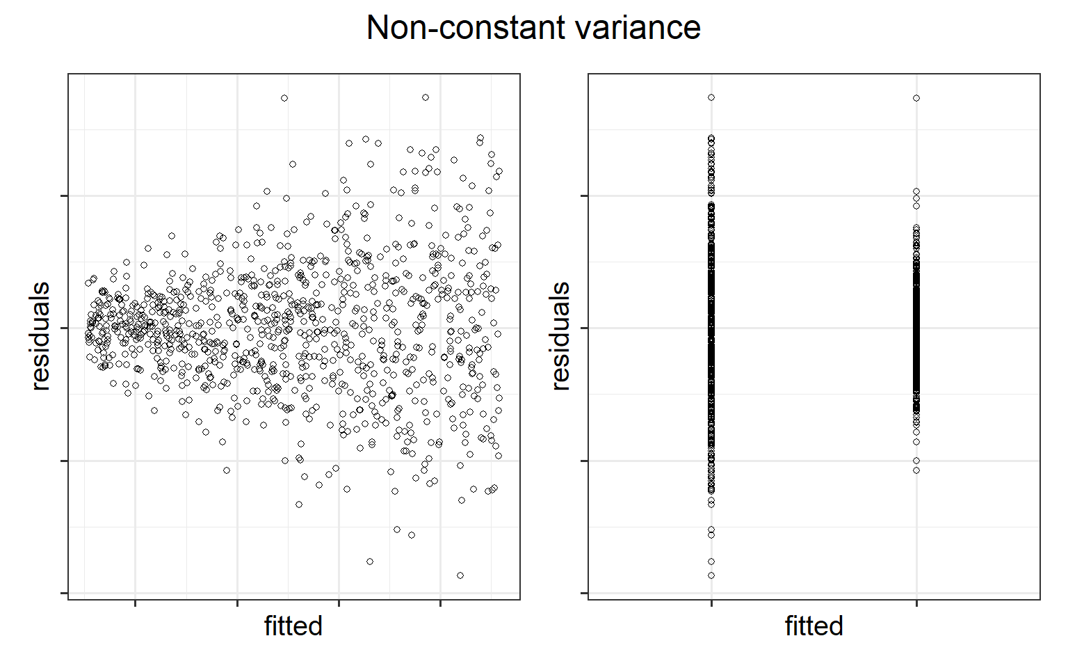
Figure 3: Non-constant variance for numeric and categorical x

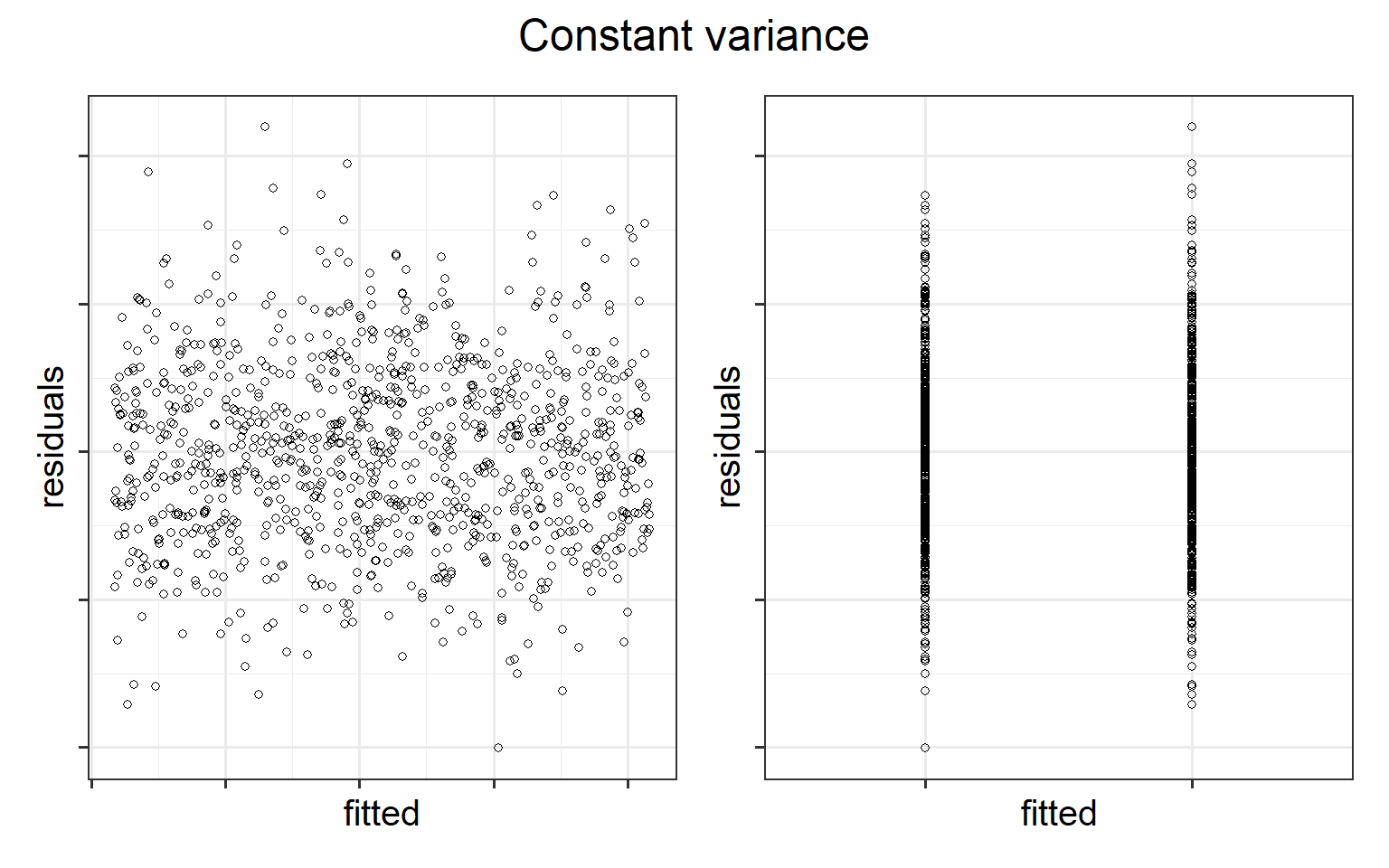
Figure 4: Constant variance for numeric and categorical x

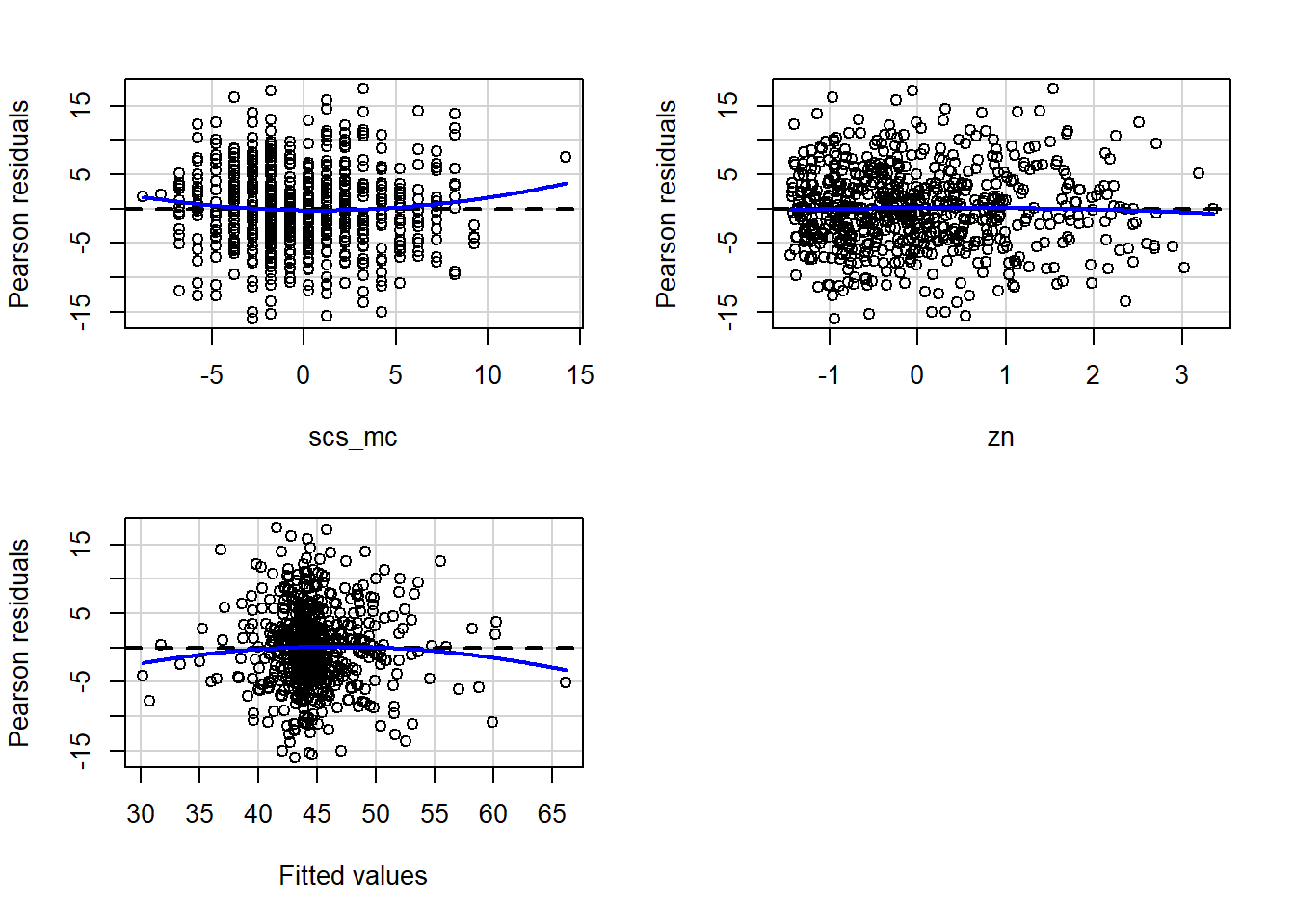
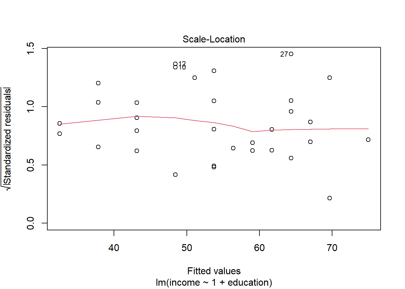
In R we can create plots of the Pearson residuals against the predicted values \(\hat y\) and against the predictors \(x_1\), … \(x_k\) by using the residualPlots() function from the car package. This function also provides the results of a lack-of-fit test for each of these relationships (note when it is the fitted values \(\hat y\) it gets called “Tukey’s test”).

Question 3

Check if the fitted models rv_mdl1 and wb_mdl1 satisfy the equal variance assumption. Use residualPlots() to plot residuals against the predictor.

Write a sentence summarising whether or not you consider the assumption to have been met for each model. Justify your answer with reference to plots.

Solution

Let’s start with our rv_mdl1 model. The vertical spread of the residuals should roughly be the same everywhere.

We can visually assess it by plotting the Pearson residuals against the fitted values:

residualPlots(rv_mdl1)

##            Test stat Pr(>|Test stat|)
## education    -0.0744           0.9412
## Tukey test   -0.0744           0.9407

Quick Tip: As the residuals can be positive or negative, we can make it easier to assess equal spread by improving the ‘resolution’ of the points.

We can make all residuals positive by discarding the sign (take the absolute value), and then take the square root to make them closer to each other.

A plot of \(\sqrt{|\text{Standardized residuals}|}\) against the fitted values is shown below:

plot(rv_mdl1, which = 3)

The plot above has the points closer to each other, and all above 0. The line seems to be relatively flat (as it should be if the spread was constant).

The spread of the standardized residuals appears to be constant as the fitted values vary.

Now for our wb_mdl1 model:

#plot
residualPlots(wb_mdl1)

##              Test stat Pr(>|Test stat|)
## outdoor_time   -0.3478           0.7306
## social_int     -0.1068           0.9157
## Tukey test     -0.4189           0.6753

Partial residual plots show no clear non-linear trends between residuals and predictors.

Visual inspection of suggested little sign of non-constant variance.

Independence

The ‘independence of errors’ assumption is the condition that the errors do not have some underlying relationship which is causing them to influence one another.

There are many sources of possible dependence, and often these are issues of study design. For example, we may have groups of observations in our data which we would expect to be related (e.g., multiple trials from the same participant). Our modelling strategy would need to take this into account.
One form of dependence is autocorrelation - this is when observations influence those adjacent to them. It is common in data for which time is a variable of interest (e.g, the humidity today is dependent upon the rainfall yesterday).

Question 4

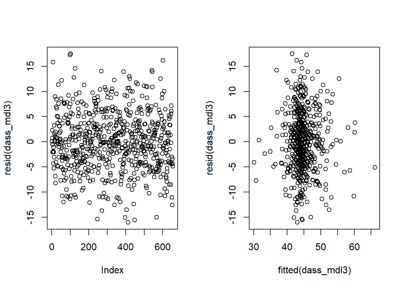
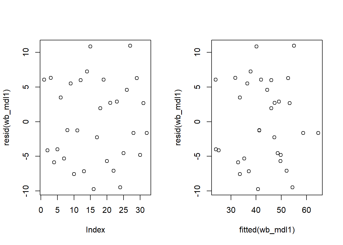
For both rv_mdl1 and wb_mdl1, visually assess whether there is autocorrelation in the error terms.

Write a sentence summarising whether or not you consider the assumption of independence to have been met for each (you may have to assume certain aspects of the study design).

Solution

Lets assess our rv_mdl1 first.

To get a single figure made up of 2 by 1 panels, you can use the command par(mfrow = c(1,2)). Then create the plot. Then you need to go back to a single figure made up by a single panel with the command par(mfrow = c(1,1)).

par(mfrow = c(1,2))
plot(resid(rv_mdl1))
plot(fitted(rv_mdl1), resid(rv_mdl1))

par(mfrow = c(1,1))

The plot of the residuals vs their index shows no clear dependence (if they were collected over time, for example, and there was an increasing trend this would highlight a violation). The residuals vs fitted plot shows that there is no association between the errors and the model predictions.

And now our wb_mdl1:

par(mfrow = c(1,2))
plot(resid(wb_mdl1))
plot(fitted(wb_mdl1), resid(wb_mdl1))

par(mfrow = c(1,1))

Similarly to above, the plot of the residuals vs their index shows no clear dependence, and the residuals vs fitted plot shows that there is no association between the errors and the model predictions.

Normality of errors

The normality assumption is the condition that the errors \(\epsilon\) are normally distributed in the population.

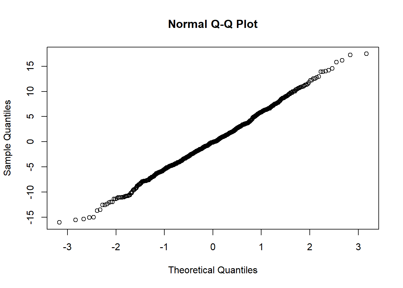
We can visually assess this condition through histograms, density plots, and quantile-quantile plots (QQplots) of our residuals \(\hat \epsilon\).

Question 5

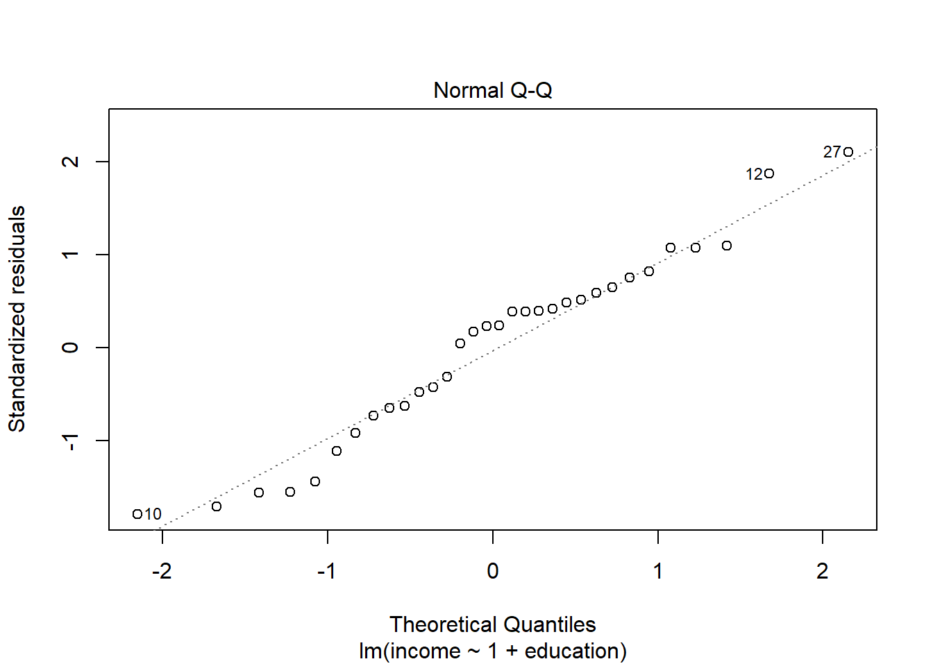
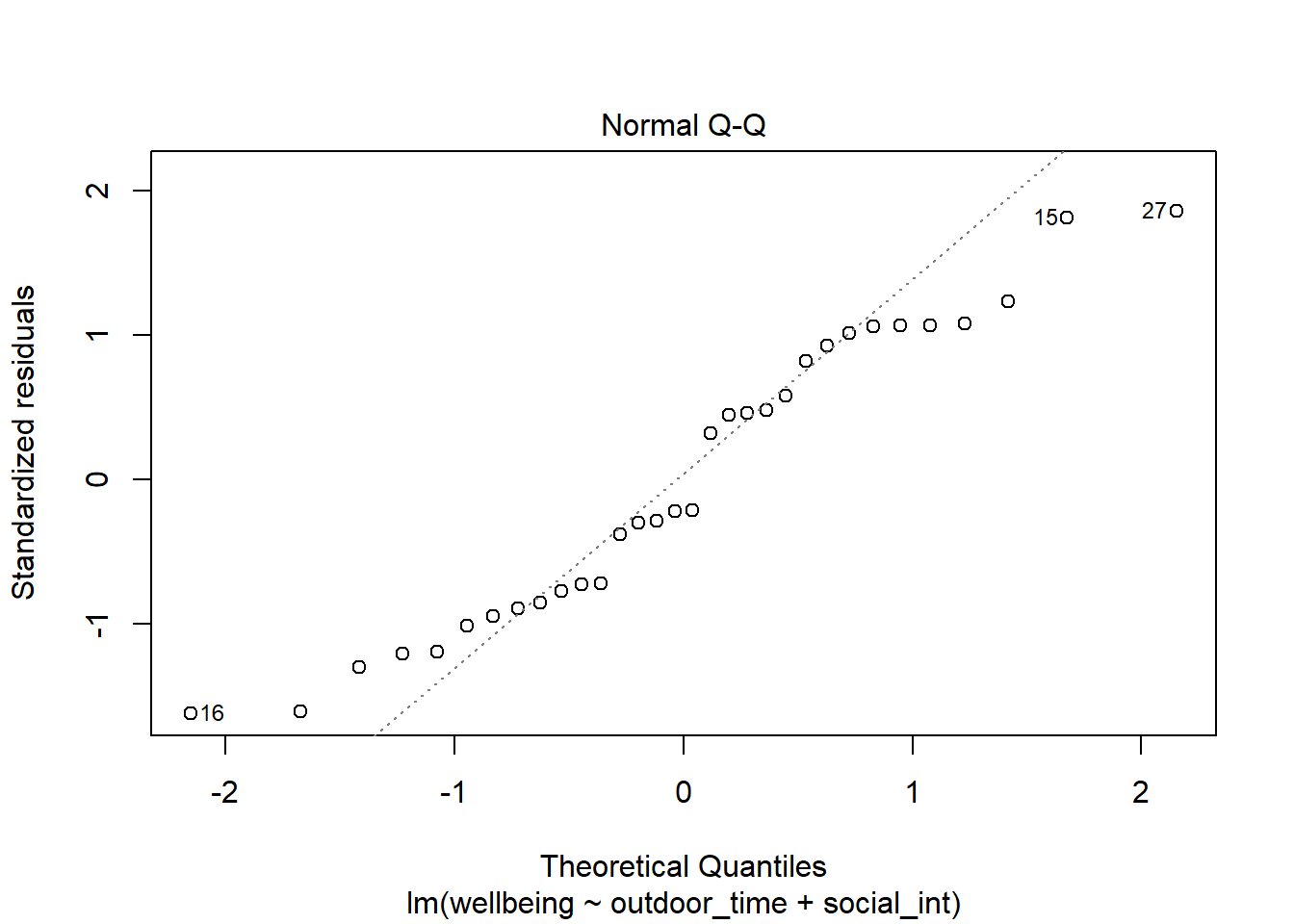
Assess the normality assumption by producing a qqplot of the residuals (either manually or using plot(model, which = ???)) for both rv_mdl1 and wb_mdl1.

Write a sentence summarising whether or not you consider the assumption to have been met. Justify your answer with reference to the plots.

Solution

We can get the QQplot from one of the plot(model) plot. Remember that departures from a linear trend in QQ plots indicate a lack of normality.

First, lets check our rv_mdl1:

plot(rv_mdl1, which = 2)

The normal quantile plot follows a linear pattern and does not highlight any substantial skew or departure from normality.

---

Now onto wb_mdl1:

plot(wb_mdl1, which = 2)

The QQplot indicates that the residuals follow close to a normal distribution. Although there is some evidence of heavier tails, given the small sample size (n=32) it is not of concern and we can be more conservative in our visual assessment of the plot.

Multicollinearity

For the linear model with multiple explanatory variables, we need to also think about multicollinearity - this is when two (or more) of the predictors in our regression model are moderately or highly correlated.

We can assess multicollinearity using the variance inflation factor (VIF), which for a given predictor \(x_j\) is calculated as:
\[ VIF_j = \frac{1}{1-R_j^2} \\ \] Suggested cut-offs for VIF are varied. Some suggest 10, others 5. Define what you will consider an acceptable value prior to calculating it. You could loosely interpret VIF values larger than 5 as moderate multicollinearity and values larger than 10 as severe multicollinearity.

In R, the vif() function from the car package will provide VIF values for each predictor in your model.

Question 6

Calculate the variance inflation factor (VIF) for the predictors in the model.

Write a sentence summarising whether or not you consider multicollinearity to be a problem here.

Solution

vif(wb_mdl1)

## outdoor_time   social_int 
##      1.13023      1.13023

The VIF values for all predictors are <5, indicating that multicollinearity is not adversely affecting model estimates.

Individual Case Diagnostics

We have seen in the case of the simple linear regression that individual cases in our data can influence our model more than others. We know about:

• Regression outliers: A large residual \(\hat \epsilon_i\) - i.e., a big discrepancy between their predicted y-value and their observed y-value.
  • Standardised residuals: For residual \(\hat \epsilon_i\), divide by the estimate of the standard deviation of the residuals. In R, the rstandard() function will give you these
  • Studentised residuals: For residual \(\hat \epsilon_i\), divide by the estimate of the standard deviation of the residuals excluding case \(i\). In R, the rstudent() function will give you these.
• High leverage cases: These are cases which have considerable potential to influence the regression model (e.g., cases with an unusual combination of predictor values).
  • Hat values: are used to assess leverage. In R, The hatvalues() function will retrieve these.
• High influence cases: When a case has high leverage and is an outlier, it will have a large influence on the regression model.
  • Cook’s Distance: combines leverage (hatvalues) with outlying-ness to capture influence. In R, the cooks.distance() function will provide these. Alongside Cook’s Distance, we can examine the extent to which model estimates and predictions are affected when an entire case is dropped from the dataset and the model is refitted.
    
• DFFit: the change in the predicted value at the \(i^{th}\) observation with and without the \(i^{th}\) observation is included in the regression.
  
• DFbeta: the change in a specific coefficient with and without the \(i^{th}\) observation is included in the regression.
  
• DFbetas: the change in a specific coefficient divided by the standard error, with and without the \(i^{th}\) observation is included in the regression.
  
• COVRATIO: measures the effect of an observation on the covariance matrix of the parameter estimates. In simpler terms, it captures an observation’s influence on standard errors.

You can get a whole bucket-load of these measures with the influence.measures() function:

• influence.measures(my_model) will give you out a dataframe of the various measures.
• summary(influence.measures(my_model)) will provide a nice summary of what R deems to be the influential points.

For questions 8-12, we will be working with our wb_mdl1 only. Feel free to apply the below to your rv_mdl1 too as as extra practice.

Question 7

Create a new tibble which contains:

1. The original variables from the model (Hint, what does wb_mdl1$model give you?)
2. The fitted values from the model \(\hat y\)
   
3. The residuals \(\hat \epsilon\)
4. The studentised residuals
5. The hat values
6. The Cook’s Distance values.

Solution

mdl_diagnost <- 
  tibble(
  wb_mdl1$model,
  fitted = fitted(wb_mdl1),
  resid = residuals(wb_mdl1),
  studres = rstudent(wb_mdl1),
  hats = hatvalues(wb_mdl1),
  cooksd = cooks.distance(wb_mdl1)
)

Question 8

Looking at the studentised residuals, are there any outliers?

Solution

In a standard normal distribution, 95% of the values are roughly between -2 and 2.

Because of this, studentised residuals of \(>2\) or \(< -2\) indicate potential outlyingness.

We can ask R whether the absolute values are \(>2\):

abs(mdl_diagnost$studres) > 2

##     1     2     3     4     5     6     7     8     9    10    11    12    13 
## FALSE FALSE FALSE FALSE FALSE FALSE FALSE FALSE FALSE FALSE FALSE FALSE FALSE 
##    14    15    16    17    18    19    20    21    22    23    24    25    26 
## FALSE FALSE FALSE FALSE FALSE FALSE FALSE FALSE FALSE FALSE FALSE FALSE FALSE 
##    27    28    29    30    31    32 
## FALSE FALSE FALSE FALSE FALSE FALSE

We could filter our newly created tibble to these observations:

mdl_diagnost %>% 
  filter(abs(studres)>2)

## # A tibble: 0 x 8
## # ... with 8 variables: wellbeing <dbl>, outdoor_time <dbl>, social_int <dbl>,
## #   fitted <dbl>, resid <dbl>, studres <dbl>, hats <dbl>, cooksd <dbl>

There are zero rows.

Question 9

Looking at the hat values, are there any observations with high leverage?

Solution

Recall from the lectures, hat values of more than \(2 \bar{h}\) (2 times the average hat value) are considered high leverage.

The average hat value, \(\bar{h}\) is calculated as \(\frac{k + 1}{n}\), where \(k\) is the number of predictors, and \(n\) is the sample size. For our model: \[ \bar h = \frac{k+1}{n} = \frac{2+1}{32} = \frac{3}{32} = 0.094 \]

We can ask whether any of observations have hat values which are greater than \(2 \bar h\):

mdl_diagnost %>%
  filter(hats > (2*0.094))

## # A tibble: 0 x 8
## # ... with 8 variables: wellbeing <dbl>, outdoor_time <dbl>, social_int <dbl>,
## #   fitted <dbl>, resid <dbl>, studres <dbl>, hats <dbl>, cooksd <dbl>

Note that 0 observations have high leverage.

Question 10

Looking at the Cook’s Distance values, are there any highly influential points?
You can also display these graphically using plot(model, which = 4) and plot(model, which = 5).

Solution

Recall from the lectures that we have a Cook’s Distance cut-off of \(\frac{4}{n-k-1}\), where \(k\) is the number of predictors, and \(n\) is the sample size.
For our model: \[ D_{cutoff} = \frac{4}{n-k-1} = \frac{4}{32 - 2 - 1} = \frac{4}{29} = 0.138 \]

There are no observations which have a high influence on our model estimates:

mdl_diagnost %>%
  filter(cooksd > 0.138)

## # A tibble: 0 x 8
## # ... with 8 variables: wellbeing <dbl>, outdoor_time <dbl>, social_int <dbl>,
## #   fitted <dbl>, resid <dbl>, studres <dbl>, hats <dbl>, cooksd <dbl>

Question 11

Use the function influence.measures() to extract these delete-1 measures of influence.

Try plotting the distributions of some of these measures.

Tip: the function influence.measures() returns an infl-type object. To plot this, we need to find a way to extract the actual numbers from it.
What do you think names(influence.measures(wb_mdl1)) shows you? How can we use influence.measures(wb_mdl1)$<insert name here> to extract the matrix of numbers?

Solution

influence.measures(wb_mdl1)

## Influence measures of
##   lm(formula = wellbeing ~ outdoor_time + social_int, data = wbdata) :
## 
##      dfb.1_ dfb.otd_ dfb.scl_   dffit cov.r   cook.d    hat inf
## 1   0.43653 -0.11116 -0.32167  0.4477 1.157 0.066470 0.1489    
## 2  -0.28160  0.03170  0.22954 -0.2917 1.225 0.028838 0.1414    
## 3   0.29581  0.07604 -0.29025  0.3540 1.088 0.041520 0.0967    
## 4  -0.26445 -0.13055  0.29341 -0.3508 1.117 0.040991 0.1071    
## 5  -0.27084  0.22733  0.10472 -0.3290 1.279 0.036700 0.1766    
## 6   0.12462 -0.02693 -0.08288  0.1460 1.141 0.007277 0.0604    
## 7  -0.17361 -0.03392  0.15313 -0.2235 1.087 0.016770 0.0597    
## 8  -0.02879 -0.07259  0.06069 -0.0918 1.309 0.002906 0.1556    
## 9   0.16925  0.08820 -0.17834  0.2477 1.088 0.020553 0.0668    
## 10 -0.24768  0.33112 -0.00551 -0.4267 1.027 0.059217 0.0956    
## 11 -0.02018 -0.02535  0.02534 -0.0492 1.166 0.000834 0.0518    
## 12  0.04644  0.38731 -0.22045  0.4474 1.164 0.066462 0.1517    
## 13 -0.15606  0.21587 -0.02477 -0.3135 1.017 0.032241 0.0626    
## 14  0.13390 -0.31537  0.10705  0.3905 1.039 0.049887 0.0899    
## 15  0.14774 -0.25595  0.08688  0.4273 0.815 0.055918 0.0487    
## 16 -0.11881  0.17855 -0.06061 -0.3502 0.873 0.038519 0.0422    
## 17  0.00121 -0.07684  0.02608 -0.1031 1.177 0.003653 0.0703    
## 18  0.00329  0.04637 -0.01574  0.0739 1.159 0.001877 0.0516    
## 19  0.04301 -0.15310  0.09227  0.2432 1.055 0.019693 0.0546    
## 20  0.05819 -0.10961 -0.03803 -0.2189 1.065 0.016025 0.0508    
## 21 -0.01498  0.00131  0.03428  0.0875 1.131 0.002622 0.0380    
## 22  0.12553 -0.15510 -0.09098 -0.3084 1.020 0.031247 0.0622    
## 23 -0.03324 -0.00580  0.05840  0.1049 1.138 0.003770 0.0466    
## 24  0.24606 -0.23731 -0.18568 -0.4783 0.911 0.071967 0.0774    
## 25  0.06123  0.10878 -0.16017 -0.2209 1.131 0.016498 0.0771    
## 26 -0.02732 -0.29363  0.23790  0.3643 1.243 0.044752 0.1666    
## 27 -0.30514  0.33726  0.20108  0.5966 0.830 0.108234 0.0858    
## 28  0.06176 -0.07036 -0.03455 -0.1080 1.263 0.004013 0.1280    
## 29 -0.15327 -0.04611  0.23001  0.3039 1.067 0.030646 0.0754    
## 30  0.11226  0.25745 -0.30386 -0.3826 1.238 0.049262 0.1686    
## 31 -0.07637 -0.05313  0.12879  0.1542 1.214 0.008153 0.1047    
## 32  0.10249 -0.07000 -0.07662 -0.1399 1.353 0.006736 0.1864   *

Let’s plot the distribution of COVRATIO statistics.
Recall that values which are \(>1+\frac{3(k+1)}{n}\) or \(<1-\frac{3(k+1)}{n}\) are considered as having strong influence.
For our model: \[ 1 \pm \frac{3(k+1)}{n} \quad = \quad 1 \pm\frac{3(2+1)}{32} \quad = \quad 1\pm \frac{9}{32} \quad = \quad 1\pm0.28 \]

The “infmat” bit of an infl-type object contains the numbers. To use it with ggplot, we will need to turn it into a dataframe (as.data.frame()), or a tibble (as_tibble()):

infdata <- influence.measures(wb_mdl1)$infmat %>%
  as_tibble()

ggplot(data = infdata, aes(x = cov.r)) + 
  geom_histogram() +
  geom_vline(aes(xintercept = c(1-0.28)))+
  geom_vline(aes(xintercept = c(1+0.28)))

It looks like a few observations may be having quite a high influence here. This is perhaps not that surprising as we only have 32 datapoints.

---

---

Less guided exercises - extra practice

Question 12

Create a new section header in your Rmarkdown document, as we are moving onto a different dataset.

The code below loads the dataset of 656 participants’ scores on Big 5 Personality traits, perceptions of social ranks, and scores on a depression and anxiety scale.

scs_study <- read_csv("https://uoepsy.github.io/data/scs_study.csv")

1. Fit the following interaction model:
   • \(\text{DASS-21 Score} = \beta_0 + \beta_1 \cdot \text{SCS Score} + \beta_2 \cdot \text{Neuroticism} + \beta_3 \cdot \text{SCS score} \cdot \text{Neuroticism} + \epsilon\)
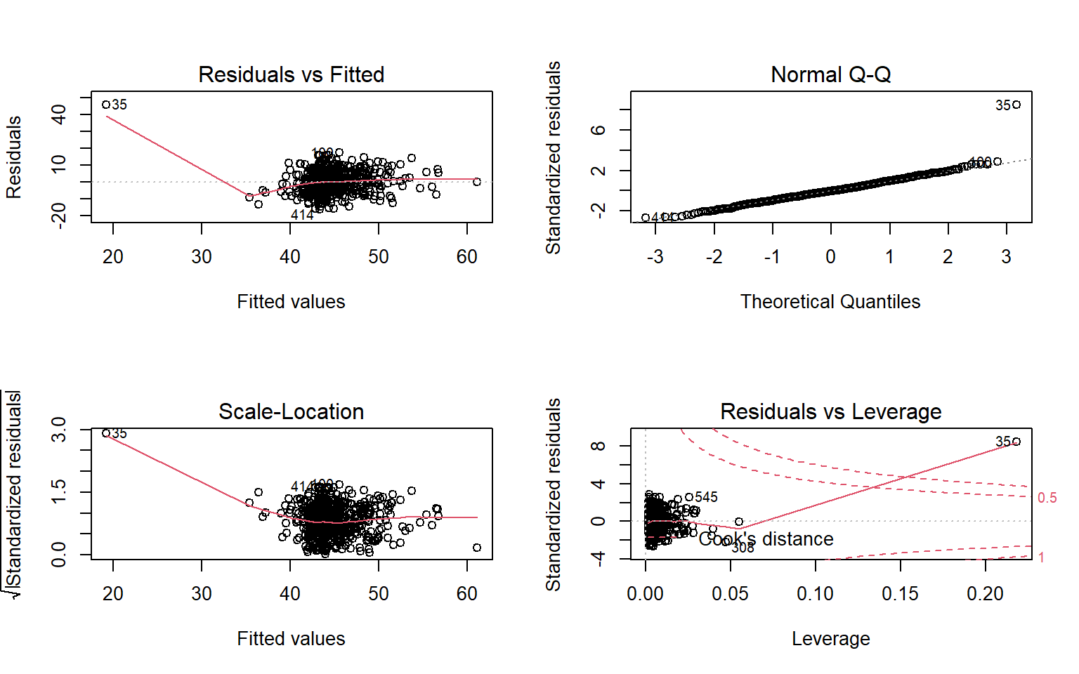
2. Check that the model meets the assumptions of the linear model (Tip: to get a broad overview you can pass your model to the plot() function to get a series of plots).
3. If you notice any violated assumptions:
   • address the issues by, e.g., excluding observations from the analysis, or replacing outliers with the next most extreme value (Winsorisation).
   • after fitting a new model which you hope addresses violations, you need to check all of your assumptions again. It can be an iterative process, and the most important thing is that your final model (the one you plan to use) meets all the assumptions.

---

Tips:

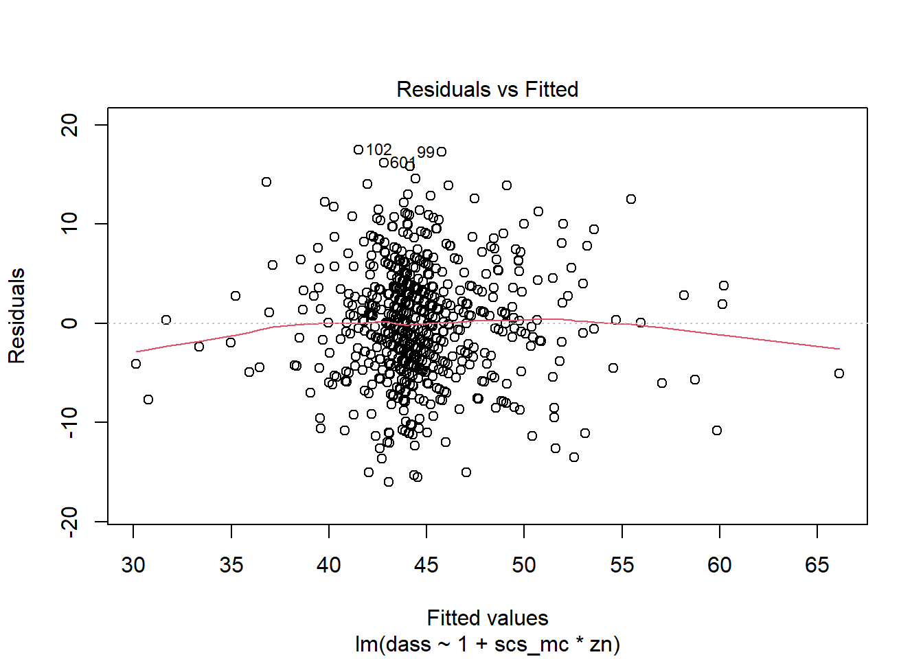
• When there is an interaction in the model, assessing linearity becomes difficult. In fact, crPlots() will not work. To assess, you can create a residuals-vs-fitted plot like we saw in the guided exercises above.
  
• Interaction terms often result in multicollinearity, because these terms are made up of the product of some ‘main effects.’ Mean-centering the variables like we have here will reduce this source of structural multicollinearity (“structural” here refers to the fact that multicollinearity is due to our model specification, rather than the data itself)
  
• You can fit a model and exclude specific observations. For instance, to remove the 3rd and 5th rows of the dataset: lm(y ~ x1 + x2, data = dataset[-c(3,5),]). Be careful to remember that these values remain in the dataset, they have simply been excluded from the model fit.

Solution

We’re going to mean-center the scs variable from the outset.

scs_study <- read_csv("https://uoepsy.github.io/data/scs_study.csv")  

scs_study <-
  scs_study %>%
  mutate(
    scs_mc = scs - mean(scs)
  )

dass_mdl2 <- lm(dass ~ 1 + scs_mc * zn, data = scs_study)

plot(dass_mdl2)

From quick visual inspection, it looks like there is at least one very influential point, which has been labelled for us as case number 35.

scs_study[35, ]

## # A tibble: 1 x 8
##      zo    zc    ze     za    zn   scs  dass scs_mc
##   <dbl> <dbl> <dbl>  <dbl> <dbl> <dbl> <dbl>  <dbl>
## 1 0.645 -1.49 0.970 -0.121  2.24    54    65   18.2

The code below fits a new model and assigns it the name dass_mdl3. How is it different from the previous model?

dass_mdl3 <- lm(dass ~ 1 + scs_mc * zn, data = scs_study[-35, ])

Does this new model meet the assumptions of multiple regression?

Linearity

plot(dass_mdl3, which = 1)

Equal variances (Homoscedasticity)

residualPlots(dass_mdl3)

##            Test stat Pr(>|Test stat|)
## scs_mc        1.6260           0.1044
## zn           -0.5074           0.6121
## Tukey test   -1.3170           0.1878

Independence of errors

par(mfrow = c(1,2))
plot(resid(dass_mdl3))
plot(fitted(dass_mdl3), resid(dass_mdl3))

par(mfrow = c(1,1))

Normality

qqnorm(resid(dass_mdl3))

Check for multicollinearity

vif(dass_mdl3)

##    scs_mc        zn scs_mc:zn 
##  1.010026  1.010174  1.000240