Model Comparison
LEARNING OBJECTIVES
- Understand measures of model fit using F.
- Understand the principles of model selection and how to compare models via F tests.
- Understand AIC and BIC.
Model Fit
F-ratio
As in simple linear regression, the F-ratio is used to test the null hypothesis that all regression slopes are zero.
It is called the F-ratio because it is the ratio of the how much of the variation is explained by the model (per paramater) versus how much of the variation is unexplained (per remaining degrees of freedom).
\[ F_{df_{model},df_{residual}} = \frac{MS_{Model}}{MS_{Residual}} = \frac{SS_{Model}/df_{Model}}{SS_{Residual}/df_{Residual}} \\ \quad \\ \begin{align} & \text{Where:} \\ & df_{model} = k \\ & df_{error} = n-k-1 \\ & n = \text{sample size} \\ & k = \text{number of explanatory variables} \\ \end{align} \]
In R, at the bottom of the output of summary(<modelname>), you can view the F-ratio, along with an hypothesis test against the alternative hypothesis that the at least one of the coefficients \(\neq 0\) (under the null hypothesis that all coefficients = 0, the ratio of explained:unexplained variance should be approximately 1):
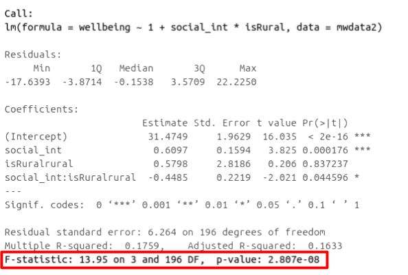
Figure 1: Multiple regression output in R, summary.lm(). F statistic highlighted
Run the code below. It reads in the wellbeing/rurality study data, and creates a new binary variable which specifies whether or not each participant lives in a rural location.
library(tidyverse)
mwdata2<-read_csv("https://uoepsy.github.io/data/wellbeing_rural.csv")
mwdata2 <-
  mwdata2 %>% mutate(
  isRural = ifelse(location=="rural","rural","notrural")
)
Fit the following model, and assign it the name “wb_mdl1.”
\(\text{Wellbeing} = \beta_0 + \beta_1 \cdot \text{Social Interactions} + \beta_2 \cdot \text{IsRural} + \epsilon\)
Model Comparison
Incremental F-test
If (and only if) two models are nested, can we compare them using an incremental F-test.
What does nested mean?
Consider that you have two regression models where Model 1 contains a subset of the predictors containted in the other Model 2 and is fitted to the same data. More simply, Model 2 contains all of the predictors included in Model 1, plus additional predictor(s). This means that Model 1 is nested within Model 2, or that Model 1 is a submodel of Model 2. These two terms, at least in this setting, are interchangeable - it might be easier to think of Model 1 as your null and Model 2 as your alternative.
What is an incremental F-test?
This is a formal test of whether the additional predictors provide a better fitting model.
Formally this is the test of:
- \(H_0:\) coefficients for the added/ommitted variables are all zero.
- \(H_1:\) at least one of the added/ommitted variables has a coefficient that is not zero.
The F-ratio for comparing the residual sums of squares between two models can be calculated as:
\[ F_{(df_R-df_F),df_F} = \frac{(SSR_R-SSR_F)/(df_R-df_F)}{SSR_F / df_F} \\ \quad \\ \begin{align} & \text{Where:} \\ & SSR_R = \text{residual sums of squares for the restricted model} \\ & SSR_F = \text{residual sums of squares for the full model} \\ & df_R = \text{residual degrees of freedom from the restricted model} \\ & df_F = \text{residual degrees of freedom from the full model} \\ \end{align} \]
Comparing regression models with anova()
Remember that you want your models to be parsimonious, or in other words, only as complex as they need to be in order to describe the data well. This means that you need to be able to justify your model choice, and one way to do so is by comparing models via anova(). If your model with multiple IVs does not provide a significantly better fit to your data than a more simplistic model with less IVs, then the more simplistic model should be preferred.
In R, we can conduct an incremental F-test by constructing two linear regression models, and passing them to the anova() function: anova(model1, model2).
If the p-value is sufficiently low (i.e., below your predetermined significance level - usually .05), then you would conclude that model 2 is significantly better fitting than model 1. If p is not < .05, then you should favour the more simplistic model.
The F-ratio you see at the bottom of summary(model) is actually a comparison between two models: your model (with some explanatory variables in predicting \(y\)) and the null model. In regression, the null model can be thought of as the model in which all explanatory variables have zero regression coefficients. It is also referred to as the intercept-only model, because if all predictor variable coefficients are zero, then the only we are only estimating \(y\) via an intercept (which will be the mean - \(\bar y\)).
Use the code below to fit the null model.
Then, use the anova() function to perform a model comparison between your earlier model (wb_mdl1) and the null model. Remember that the null model tests the null hypothesis that all beta coefficients are zero. By comparing null_model to wb_mdl1, we can test whether we should include the two IVs of social_int and isRural.
Check that the F-statistic and the p-value are the the same as that which is given at the bottom of summary(wb_mdl1).
null_model <- lm(wellbeing ~ 1, data = mwdata2)
Does weekly outdoor time explain a significant amount of variance in wellbeing scores over and above weekly social interactions and location (rural vs not-rural)?
Provide an answer to this question by fitting and comparing two models (one of them you may already have fitted in an earlier question).
Recall the data on Big 5 Personality traits, perceptions of social ranks, and depression and anxiety scale scores:
scs_study <- read_csv("https://uoepsy.github.io/data/scs_study.csv")
summary(scs_study)
## zo zc ze za
## Min. :-2.81928 Min. :-3.21819 Min. :-3.00576 Min. :-2.94429
## 1st Qu.:-0.63089 1st Qu.:-0.66866 1st Qu.:-0.68895 1st Qu.:-0.69394
## Median : 0.08053 Median : 0.00257 Median :-0.04014 Median :-0.01854
## Mean : 0.09202 Mean : 0.01951 Mean : 0.00000 Mean : 0.00000
## 3rd Qu.: 0.80823 3rd Qu.: 0.71215 3rd Qu.: 0.67085 3rd Qu.: 0.72762
## Max. : 3.55034 Max. : 3.08015 Max. : 2.80010 Max. : 2.97010
## zn scs dass
## Min. :-1.4486 Min. :27.00 Min. :23.00
## 1st Qu.:-0.7994 1st Qu.:33.00 1st Qu.:41.00
## Median :-0.2059 Median :35.00 Median :44.00
## Mean : 0.0000 Mean :35.77 Mean :44.72
## 3rd Qu.: 0.5903 3rd Qu.:38.00 3rd Qu.:49.00
## Max. : 3.3491 Max. :54.00 Max. :68.00Research questions
Part 1: Beyond Neuroticism and its interaction with social comparison, does Openness predict symptoms of depression, anxiety and stress?
Part 2: Beyond Neuroticism and its interaction with social comparison, do other personality traits predict symptoms of depression, anxiety and stress?
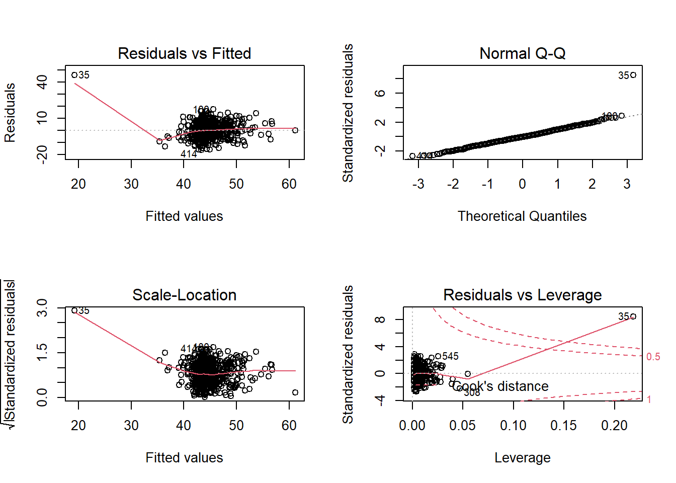
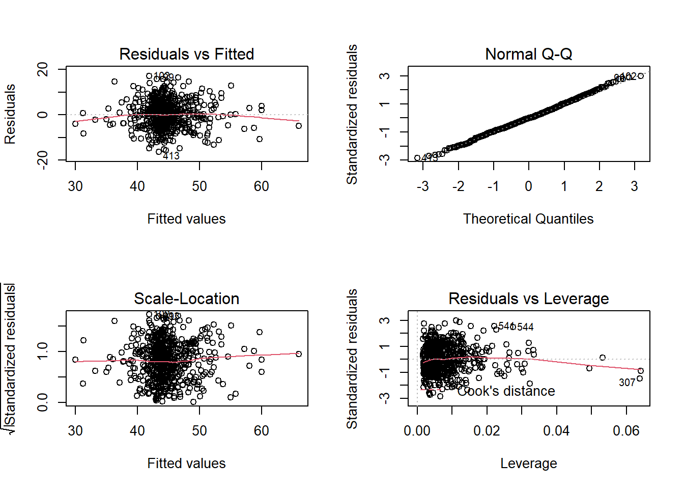
Construct and compare multiple regression models to answer these two question. Remember to check that your models meet assumptions (for this exercises, a quick eyeball of the diagnostic plots will suffice. Were this an actual research project, you would want to provide a more thorough check, for instance conducting formal tests of the assumptions).
Although the solutions are available immediately for this question, we strongly advocate that you attempt it yourself before looking at them.


AIC & BIC
If models are not nested, we cannot compare them using an incremental F-test. Instead, for non-nested models, we can use information criterion statistics, such as AIC and BIC.
What does non-nested mean?
Consider that you have two regression models where Model 1 contains different variables to those contained in Model 2, where both models are fitted to the same data. More simply, Model 1 and Model 2 contain unique variables that are not shared. This means that Model 1 and Model 2 are not nested.
What are AIC & BIC?
AIC (Akaike Information Criterion) and BIC (Bayesian Information Criterion) combine information about the sample size, the number of model parameters, and the residual sums of squares (\(SS_{residual}\)). Models do not need to be nested to be compared via AIC and BIC, but they need to have been fit to the same dataset.
For both of these fit indices, lower values are better, and both include a penalty for the number of predictors in the model (although BIC’s penalty is harsher):
\[ AIC = n\,\text{ln}\left( \frac{SS_{residual}}{n} \right) + 2k \\ \quad \\ BIC = n\,\text{ln}\left( \frac{SS_{residual}}{n} \right) + k\,\text{ln}(n) \\ \quad \\ \begin{align} & \text{Where:} \\ & SS_{residual} = \text{sum of squares residuals} \\ & n = \text{sample size} \\ & k = \text{number of explanatory variables} \\ & \text{ln} = \text{natural log function} \end{align} \]
In R, we can calculate AIC and BIC by using the AIC() and BIC() functions.
Lets compare the AIC and BIC values of two models, each looking at the associations of DASS scores and two personality traits. Fit the following models, and compare using AIC() and BIC(). Report which model you think best fits the data.
\(\text{DASS} = \beta_0 + \beta_1 \cdot \text{Neuroticism} + \beta_2 \cdot \text{Extraversion} + \epsilon\)
\(\text{DASS} = \beta_0 + \beta_1 \cdot \text{Openness} + \beta_2 \cdot \text{Agreeableness} +\epsilon\)
Choosing the Right Model Comparison Approach
The code below fits 5 different models:
model1 <- lm(wellbeing ~ social_int + outdoor_time, data = mwdata2)
model2 <- lm(wellbeing ~ social_int + outdoor_time + age, data = mwdata2)
model3 <- lm(wellbeing ~ social_int + outdoor_time + routine, data = mwdata2)
model4 <- lm(wellbeing ~ social_int + outdoor_time + routine + age, data = mwdata2)
model5 <- lm(wellbeing ~ social_int + outdoor_time + routine + steps_k, data = mwdata2)
For each of the below pairs of models, what methods are/are not available for us to use for comparison and why?
model1vsmodel2model2vsmodel3model1vsmodel4model3vsmodel5
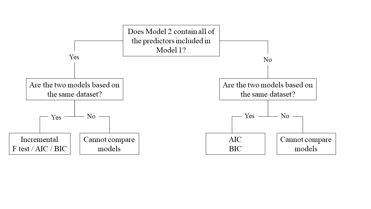
This flowchart might help you to reach your decision:
Extra reading: Joshua Loftus’ Blog: Model selection bias invalidates significance tests