Contrasts, Study Design, & Factorial ANOVA

LEARNING OBJECTIVES

1. Understand how to specify contracts to test specific effects.
   
2. Understand different types of study design.
3. Interpret interactions with effects coding.

Case Study - Contrasts

In the first section of this lab, you will be presented with a research question, and will need to go through the steps of describing, visualising, modelling, and interpreting the results.

Research Question: Does WPM differ by caffeine treatment condition?

To investigate if the number of words typed per minute (WPM) differs among caffeine treatment conditions, the researchers conducted an experiment where participants were randomly allocated to one of four treatment conditions. Two of these conditions included non-caffeinated drinks - control (water) and mint tea, and the other two caffeinated drinks - coffee and red bull.

Drink	Caffeine	Temp
Control (Water)	No	Cold
Red Bull	Yes	Cold
Coffee	Yes	Hot
Mint Tea	No	Hot

The researchers were specifically interested in the following comparisons:

• Whether having some kind of caffeine (i.e., red bull / coffee), rather than no caffeine (i.e., control - water / mint tea), resulted in a difference in average WPM
• Whether there was a difference in average WPM between those with hot drinks (i.e., mint tea / coffee) in comparison to those with cold drinks (control - water / red bull)

Caffeine data codebook.

Download link

The data is available at https://uoepsy.github.io/data/caffeinedrink.csv.
Preview

The first six rows of the data are:

treatment	wpm
control	109.43
control	113.83
control	113.22
control	110.46
control	116.23
control	113.12

Question 1

1. Load the tidyverse package.
2. Read the data into R using the function read_csv() and name the data caffeine.
3. Check for the correct coding of all variables (i.e., categorical variables should be factors and numeric variables should be numeric).

Solution

library(tidyverse)
caffeine <- read_csv("https://uoepsy.github.io/data/caffeinedrink.csv")

Treatment is a categorical variable but it is coded as a character (<chr>), so we need to correct this:

caffeine <- caffeine %>%
  mutate(treatment = as.factor(treatment))

Question 2

Numerically and visually summarise the caffeine dataset. Comment on any observed differences among treatment groups.

Solution

caffeine%>%
  group_by(treatment) %>%
  summarise(n = n(), 
            M = mean(wpm), 
            SD = sd(wpm))

## # A tibble: 4 x 4
##   treatment     n     M    SD
##   <fct>     <int> <dbl> <dbl>
## 1 coffee       10  114.  1.82
## 2 control      10  112.  1.98
## 3 mint_tea     10  111.  2.13
## 4 red_bull     10  117.  2.15

We have a continuous outcome and a categorical predictor - a boxplot would be most appropriate for visualisations:

ggplot(data = caffeine, aes(x = treatment, y = wpm, color = treatment)) +
  geom_boxplot() +
  labs(x = 'Treatment Condition', y = 'WPM') + 
    theme_classic()

From the boxplots, it seems that those in the Red Bull condition, on average, typed the most WPM, whilst those in the Mint Tea condition the fewest.

Overall, the average WPM appears to be lower for those in the non-caffeine conditions (i.e., control - water / mint tea) in comparison to those in the caffeine drinks condition (red bull / coffee).

Question 3

Set an appropriate reference group based on the research question.

Solution

It would make most sense to have the ‘Control’ caffeine treatment condition as our reference group.

caffeine$treatment <- fct_relevel(caffeine$treatment, "control")

Question 4

Fit the following model, and assign it the name “caf_mdl1.”

Examine and describe the coefficients in the output of summary() before interpreting the F-test results from anova() in the context of the ANOVA null hypothesis.

\(\text{WPM} = \beta_0 + \beta_1 \cdot \text{Treatment (Category)} + \epsilon\)

Solution

caf_mdl1 <- lm(wpm ~ treatment, data=caffeine)
summary(caf_mdl1)

## 
## Call:
## lm(formula = wpm ~ treatment, data = caffeine)
## 
## Residuals:
##    Min     1Q Median     3Q    Max 
## -3.652 -1.362 -0.151  1.125  4.729 
## 
## Coefficients:
##                   Estimate Std. Error t value Pr(>|t|)    
## (Intercept)       112.1460     0.6402 175.179  < 2e-16 ***
## treatmentcoffee     2.3350     0.9053   2.579   0.0141 *  
## treatmentmint_tea  -1.0550     0.9053  -1.165   0.2516    
## treatmentred_bull   4.5060     0.9053   4.977 1.61e-05 ***
## ---
## Signif. codes:  0 '***' 0.001 '**' 0.01 '*' 0.05 '.' 0.1 ' ' 1
## 
## Residual standard error: 2.024 on 36 degrees of freedom
## Multiple R-squared:  0.5563, Adjusted R-squared:  0.5194 
## F-statistic: 15.05 on 3 and 36 DF,  p-value: 1.651e-06

anova(caf_mdl1)

## Analysis of Variance Table
## 
## Response: wpm
##           Df Sum Sq Mean Sq F value    Pr(>F)    
## treatment  3 185.00  61.666  15.047 1.651e-06 ***
## Residuals 36 147.54   4.098                      
## ---
## Signif. codes:  0 '***' 0.001 '**' 0.01 '*' 0.05 '.' 0.1 ' ' 1

The estimate corresponding to (Intercept) contains \(\hat \beta_0 = \hat \mu_1 = 112.1460\). The estimated average WPM for those in the control condition (water) is approximately 112.15.

The next estimate corresponds to treatmentcoffee and is \(\hat \beta_2 = 2.3350\). The difference in mean WPM between Control and Coffee is estimated to be \(2.3350\). In other words, people who have had a coffee type approximately 2.3 words per minute more than those who have had water.

The estimate corresponding to treatmentmint_tea is \(\hat \beta_3 = -1.0550\). This is the estimated difference in mean WPM between Control and Mint Tea is estimated to be \(-1.0550\). In other words, people who have had a mint tea type approximately 1.1 words per minute less than those who have had water.

The estimate corresponding to treatmentred_bull is \(\hat \beta_4 = 4.5060\). This is the estimated difference in mean WPM between Control and Red Bull is estimated to be \(4.5060\). In other words, people who have had a red bull type approximately 4.5 words per minute more than those who have had water.

We performed an analysis of variance against the null hypothesis of equal population mean spending across four types of treatment condition. At the 5% significance level, we reject the null hypothesis as there is strong evidence that at least a pair of means differ from each other \(F(3, 36) = 15.05\), \(p < .001\).

As an example, suppose you are testing whether \(H_0: \mu_{A} = \mu_{B} = \mu_{C} = \mu_{D}\). If a pair of those differs, e.g. \(\mu_{C} \neq \mu_{D}\), then the claim doesn’t hold.

Question 5

The two planned comparisons that the researchers were interested in can be translated into the following research hypotheses:

\[\begin{aligned} 1. \quad H_0 &: \mu_\text{No Caffeine} = \mu_\text{Caffeine} \\ \quad H_0 &: \frac{1}{2} (\mu_\text{Control} + \mu_\text{Mint Tea}) = \frac{1}{2} (\mu_\text{Coffee} + \mu_\text{Red Bull}) \\ 2. \quad H_0 &: \mu_\text{Hot Drink} = \mu_\text{Cold Drink} \\ \quad H_0 &: \frac{1}{2} (\mu_\text{Coffee} + \mu_\text{Mint Tea}) = \frac{1}{2} (\mu_\text{Control} + \mu_\text{Red Bull}) \end{aligned}\]

After checking the levels of the factor treatment, use emmeans to obtain the estimated treatment means and uncertainties for your factor. Hint use plot() to visualise this.

Solution

levels(caffeine$treatment)

## [1] "control"  "coffee"   "mint_tea" "red_bull"

library(emmeans)
emm <- emmeans(caf_mdl1, ~ treatment)
emm

##  treatment emmean   SE df lower.CL upper.CL
##  control      112 0.64 36      111      113
##  coffee       114 0.64 36      113      116
##  mint_tea     111 0.64 36      110      112
##  red_bull     117 0.64 36      115      118
## 
## Confidence level used: 0.95

plot(emm)

Question 6

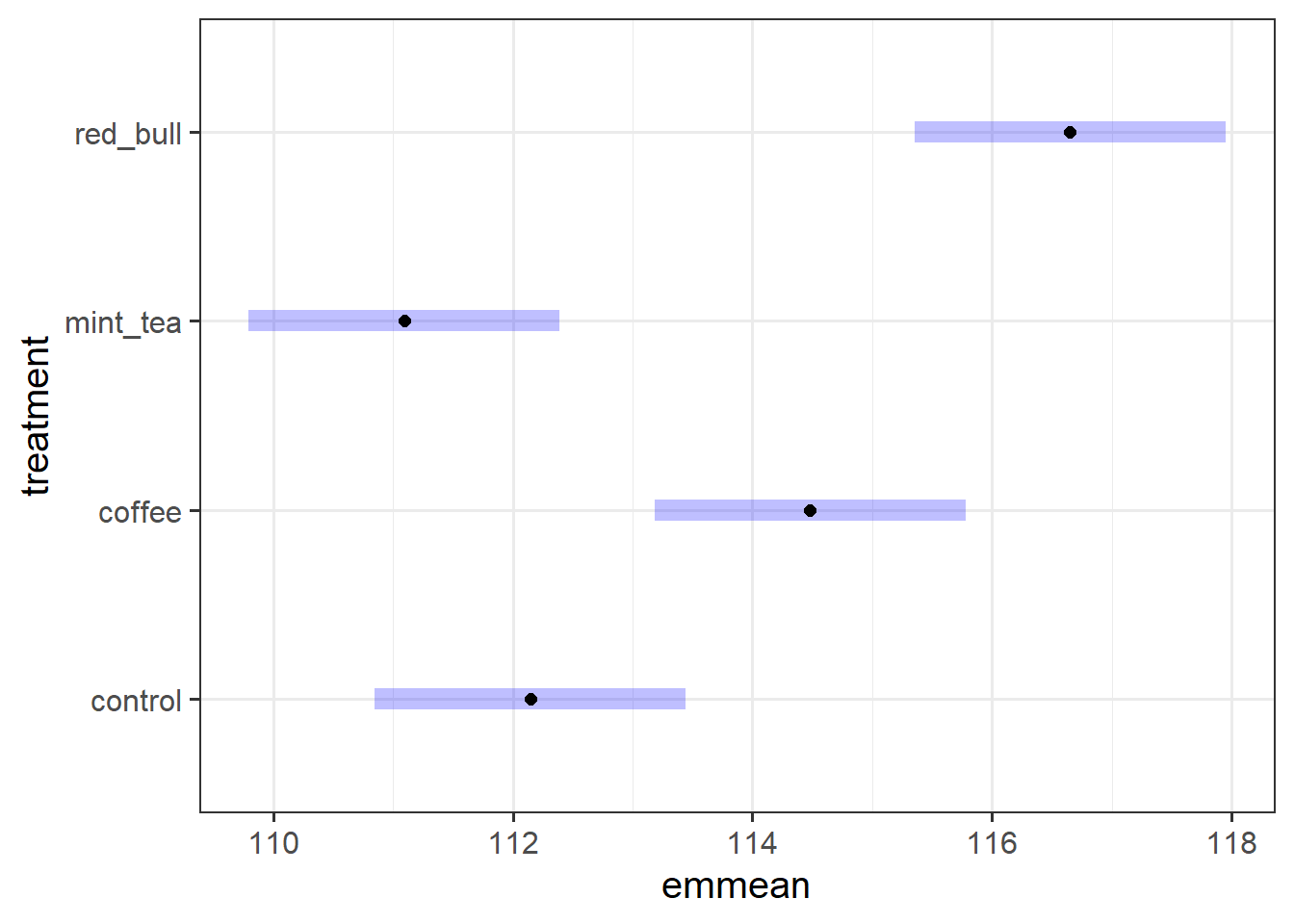
Specify the coefficients of the comparisons and run the contrast analysis. Obtain 95% confidence intervals, and then interpret your results in relation to the researchers hypotheses.

Solution

comp <- list("No Caffeine - Caffeine" = c(1/2, -1/2, 1/2, -1/2),
             "Hot Drink - Cold Drink" = c(-1/2, 1/2, 1/2, -1/2)
             )

comp_res <- contrast(emm, method = comp)
comp_res

##  contrast               estimate   SE df t.ratio p.value
##  No Caffeine - Caffeine    -3.95 0.64 36  -6.167  <.0001
##  Hot Drink - Cold Drink    -1.61 0.64 36  -2.520  0.0163

confint(comp_res)

##  contrast               estimate   SE df lower.CL upper.CL
##  No Caffeine - Caffeine    -3.95 0.64 36    -5.25   -2.650
##  Hot Drink - Cold Drink    -1.61 0.64 36    -2.91   -0.315
## 
## Confidence level used: 0.95

The hypothesis test for the first contrast could be reported as follows:

We performed a test against \(H_0: \frac{1}{2}(\mu_1 + \mu_3) - \frac{1}{2}(\mu_2 + \mu_4) = 0\). At the 5% significance level, there was evidence that the mean WPM for those who were in the no caffeine condition was significantly different from those in a caffeine condition \(t(36) = -6.17, p = < .001\) (two-sided). We are 95% confident that those who consumed no caffeine typed, on average, between 2.7 and 5.3 words less per minute than those who consumed some form of caffeine \(CI_{95}[-5.25, -2.65]\).

The hypothesis test for the second contrast could be reported as follows:

We performed a test against \(H_0: \frac{1}{2}(\mu_2 + \mu_3) - \frac{1}{2}(\mu_1 + \mu_4) = 0\). At the 5% significance level, there was evidence that the average WPM for those in the hot drink condition significantly differed from those in the cold drink condition \(t(36) = -2.52, p = .02\) (two-sided). We are 95% confident that those who consumed a hot drink typed, on average, between 0.3 and 2.9 words less per minute than those who consumed a cold drink \(CI_{95}[-2.91, -0.32]\).

Study Design

For each of the below experiment descriptions, note (1) the design, (2) number of variables of interest, (3) levels of categorical variables, (4) what you think the reference group should be and why.

Question 1

A group of researchers were interested in whether sleep deprivation influenced reaction time. They hypothesised that sleep deprived individuals would have slower reaction times than non-sleep deprived individuals.

To test this, they recruited 60 participants who were matched on a number of demographic variables including age and sex. One member of each pair (e.g., female aged 18) was placed into a different sleep condition - ‘Sleep Deprived’ (4 hours per night) or ‘Non-Sleep Deprived’ (8 hours per night).

Solution

1. Design = Between-person: Matched pairs
2. No of variables of interest = 2 - Sleep Condition and Reaction Time
3. Levels of variables = Sleep Condition has 2 levels - Sleep Deprived and Non-Sleep Deprived; Reaction Time is a continuous measure, so has no associated levels
4. Reference Groups = Sleep Condition - Non-Sleep Deprived because the RQ stated that the researchers were interested in how the sleep deprived group differed from the non-sleep deprived group.

Question 2

A group of researchers were interested in replicating an experiment testing the Stroop Effect.

They recruited 50 participants who took part in Task A (word colour and meaning are congruent) and Task B (word colour and meaning are incongruent) where they were asked to name the color of the ink instead of reading the word. The order of presentation was counterbalanced across participants. The researchers hypothesised that participants would take significantly more time (‘response time’ measured in seconds) to complete Task B than Task A.

You can test yourself here for fun: Stroop Task

Solution

1. Design = Within-person: repeated measures
2. No of variables of interest = 2 - Task and Response Time
3. Levels of variables = Task has 2 levels - A and B; Response Time is a continuous measure, so has no associated levels
4. Reference Groups = Task - A because the RQ stated that the researchers were interested in how response time in Task B differed from the response time in Task A.

Question 3

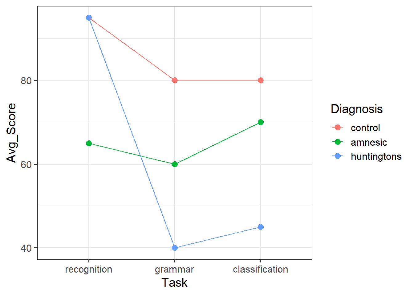
A group of researchers wanted to test a hypothesised theory according to which patients with amnesia will have a deficit in explicit memory but not implicit memory. Huntingtons patients, on the other hand, will display the opposite: they will have no deficit in explicit memory, but will have a deficit in implicit memory.

To test this, researchers designed a study that included two variables: ‘Diagnosis’ (Amnesic, Huntingtons, Control) and ‘Task’ (Grammar, Classification, Recognition) where participants were randomly assigned to a Task condition. The first two tasks (Grammar and Classification) are known to reflect implicit memory processes, whereas the Recognition task is known to reflect explicit memory processes.

Solution

1. Design = Between-person: 3×3 factorial design
2. No of variables of interest = 2 - Diagnosis and Task
3. Levels of variables = Diagnosis has 3 levels - Amnesic, Huntingtons, and Control; Task has 3 levels - Grammar, Classification, and Recognition
4. Reference Groups = Diagnosis - Control; Task - Recognition. We have chosen Control since the other two groups have some form of cognitive impairment; and the Recognition task since it measures explicit memory whilst the other two task types implicit.

Factorial ANOVA

Next week, the lab will focus on Experiment 3 described above. You have already worked with some of this data before - see semester 1 week 8 lab, but we now have a third task condition - Classification.

Data download link: https://uoepsy.github.io/data/cognitive_experiment.csv

We have data from the 45 participants (15 amnesiacs, 15 Huntington individuals, and 15 controls). Recall that study involves two factors, now with three levels each. For each combination of factor levels we have 5 observations:

	Task
Diagnosis	grammar	classification	recognition
amnesic	44, 63, 76, 72, 45	72, 66, 55, 82, 75	70, 51, 82, 66, 56
huntingtons	24, 30, 51, 55, 40	53, 59, 33, 37, 43	107, 80, 98, 82, 108
control	76, 98, 71, 70, 85	92, 65, 86, 67, 90	107, 80, 101, 82, 105

The five observations are assumed to come from a population having a specific mean. The population means corresponding to each combination of factor levels can be schematically written as:

\[ \begin{matrix} & & & \textbf{Task} & \\ & & (j=1)\text{ grammar} & (j=2)\text{ classification} & (j=3)\text{ recognition} \\ & (i=1)\text{ control} & \mu_{1,1} & \mu_{1,2} & \mu_{1,3} \\ \textbf{Diagnosis} & (i=2)\text{ amnesic} & \mu_{2,1} & \mu_{2,2} & \mu_{2,3} \\ & (i=3)\text{ huntingtons} & \mu_{3,1} & \mu_{3,2} & \mu_{3,3} \end{matrix} \]

Question 1

Repeat the steps outlined in the Semester 1 Week 8 lab, but using the new dataset.

• Read the cognitive experiment data into R.
• Convert categorical variables into factors, and assign more informative labels to the factor levels according to the data description provided above.
• Relevel the Diagnosis factor to have ‘Control’ as the reference group.
• Relevel the Task factor to have ‘Recognition’ as the reference group.
• Rename the response variable from Y to Score.
• Describe the data.
• Visualise the interaction between Diagnosis and Task.

Solution

Load the tidyverse library and read the data into R:

cog <- read_csv('https://uoepsy.github.io/data/cognitive_experiment.csv')
head(cog)

## # A tibble: 6 x 3
##   Diagnosis  Task     Y
##       <dbl> <dbl> <dbl>
## 1         1     1    44
## 2         1     1    63
## 3         1     1    76
## 4         1     1    72
## 5         1     1    45
## 6         1     2    72

We will now convert Diagnosis and Task into factors, making the labels of each factor level more meaningful.

According to the data description, the encoding of the factor Diagnosis is: 1 = amnesic patients, 2 = Huntingtons patients, and 3 are control patients.The encoding for the factor Task is: 1 = grammar task, 2 = classification task, and 3 = recognition task.

cog$Diagnosis <- factor(cog$Diagnosis, 
                        labels = c("amnesic", "huntingtons", "control"), 
                        ordered = FALSE)
cog$Task <- factor(cog$Task, 
                   labels = c("grammar", "classification", "recognition"), 
                   ordered = FALSE)

Relevel the Diagnosis factor so that the reference group is “Control”:

cog$Diagnosis <- fct_relevel(cog$Diagnosis, "control")
cog$Task <- fct_relevel(cog$Task, "recognition")

Rename the response:

cog <- cog %>%
    rename(Score = Y)

Look at the data:

head(cog)

## # A tibble: 6 x 3
##   Diagnosis Task           Score
##   <fct>     <fct>          <dbl>
## 1 amnesic   grammar           44
## 2 amnesic   grammar           63
## 3 amnesic   grammar           76
## 4 amnesic   grammar           72
## 5 amnesic   grammar           45
## 6 amnesic   classification    72

Describe data:

cog_stats <- cog %>% 
    group_by(Diagnosis, Task) %>%
    summarise(
        Avg_Score = mean(Score), 
        SD = sd(Score),
        SE = sd(Score) / sqrt(n())
        )

cog_stats

## # A tibble: 9 x 5
## # Groups:   Diagnosis [3]
##   Diagnosis   Task           Avg_Score    SD    SE
##   <fct>       <fct>              <dbl> <dbl> <dbl>
## 1 control     recognition           95  13.0  5.81
## 2 control     grammar               80  11.7  5.22
## 3 control     classification        80  13.0  5.81
## 4 amnesic     recognition           65  12.2  5.44
## 5 amnesic     grammar               60  14.9  6.67
## 6 amnesic     classification        70  10.2  4.55
## 7 huntingtons recognition           95  13.4  5.98
## 8 huntingtons grammar               40  13.2  5.92
## 9 huntingtons classification        45  10.9  4.86

Since we have not yet fitted our model, we cannot use the emmip function from emmeans or plot_model from sjPlot. We can however use a simple ggplot and use our summary scores from above:

ggplot(data = cog_stats, aes(x = Task, y = Avg_Score, color = Diagnosis)) +
    geom_point(size = 3) +
    geom_line(aes(x = as.numeric(Task)))

Control patients consistently perform best across all tasks. They don’t seem to differ substantially in their scores between grammar and classification tasks, but they clearly perform better in the recognition task than the grammar and classification ones.

Amnesic patients appear to perform better than Huntingtons patients in grammar an classification tasks (reflecting intrinsic memory processes) and perform worse than Huntingtons patients in the recognition task (reflecting extrinsic memory processes).

Question 2

The model with interaction is:

\[\begin{aligned} Score &= \beta_0 \\ &+ \beta_1 D_\text{Control} + \beta_2 D_\text{Amnesic} \\ &+ \beta_3 T_\text{Recognition} + \beta_4 D_\text{Grammar} \\ &+ \beta_5 (D_\text{Control} * T_\text{Recognition}) + \beta_6 (D_\text{Amnesic} * T_\text{Recognition}) \\ &+ \beta_7 (D_\text{Control} * T_\text{Grammar}) + \beta_8 (D_\text{Amnesic} * T_\text{Grammar}) \\ &+ \epsilon \end{aligned}\]

Fit the above model, and set the the sum to zero constraint for Diagnosis of ‘Control’ and Task of ‘Recognition.’

Applying the sum to zero constraint, we would have:

\[\begin{aligned} \text{Intercept (global mean)} &= \beta_0 \frac{\mu_{1,1} + \mu_{1,2} + \cdots + \mu_{3,3}}{9} \\ \beta_{Huntingtons} &= -(\beta_1 + \beta_2) \\ \beta_{Classification} &= -(\beta_3 + \beta_4) \\ \beta_{Huntingtons:Classification} &= -(\beta_5 + \beta_6 + \beta_7 + \beta_8) \end{aligned}\]

Solution

The fitted model should be:

contrasts(cog$Diagnosis) <- "contr.sum"
contrasts(cog$Task) <- "contr.sum"
mdl_int1 <- lm(Score ~ Diagnosis * Task, data = cog)
summary(mdl_int1)

## 
## Call:
## lm(formula = Score ~ Diagnosis * Task, data = cog)
## 
## Residuals:
##    Min     1Q Median     3Q    Max 
##    -16    -12      2     11     18 
## 
## Coefficients:
##                  Estimate Std. Error t value Pr(>|t|)    
## (Intercept)        70.000      1.872  37.384  < 2e-16 ***
## Diagnosis1         15.000      2.648   5.664 1.95e-06 ***
## Diagnosis2         -5.000      2.648  -1.888 0.067085 .  
## Task1              15.000      2.648   5.664 1.95e-06 ***
## Task2             -10.000      2.648  -3.776 0.000576 ***
## Diagnosis1:Task1   -5.000      3.745  -1.335 0.190216    
## Diagnosis2:Task1  -15.000      3.745  -4.005 0.000297 ***
## Diagnosis1:Task2    5.000      3.745   1.335 0.190216    
## Diagnosis2:Task2    5.000      3.745   1.335 0.190216    
## ---
## Signif. codes:  0 '***' 0.001 '**' 0.01 '*' 0.05 '.' 0.1 ' ' 1
## 
## Residual standard error: 12.56 on 36 degrees of freedom
## Multiple R-squared:  0.7318, Adjusted R-squared:  0.6722 
## F-statistic: 12.28 on 8 and 36 DF,  p-value: 2.844e-08

anova(mdl_int1)

## Analysis of Variance Table
## 
## Response: Score
##                Df Sum Sq Mean Sq F value    Pr(>F)    
## Diagnosis       2   5250 2625.00 16.6373  7.64e-06 ***
## Task            2   5250 2625.00 16.6373  7.64e-06 ***
## Diagnosis:Task  4   5000 1250.00  7.9225 0.0001092 ***
## Residuals      36   5680  157.78                      
## ---
## Signif. codes:  0 '***' 0.001 '**' 0.01 '*' 0.05 '.' 0.1 ' ' 1

Next week, we will explore the summary() and anova() output in detail. If you have time, note down what you think these estimates might be telling us. Remember, the interpretation of the estimates is now different from what you had in Semester 1 Week 8 - now each beta coefficient is the difference between a group mean and the overall mean.