Simple linear regression

Information about solutions

Solutions for these exercises are available immediately below each question.
We would like to emphasise that much evidence suggests that testing enhances learning, and we strongly encourage you to make a concerted attempt at answering each question before looking at the solutions. Immediately looking at the solutions and then copying the code into your work will lead to poorer learning.
We would also like to note that there are always many different ways to achieve the same thing in R, and the solutions provided are simply one approach.

Be sure to check the solutions to last week’s exercises.
You can still ask any questions about previous weeks’ materials if things aren’t clear!

LEARNING OBJECTIVES

1. Be able to specify a simple linear model.
2. Understand what fitted values and residuals are.
3. Be able to interpret the coefficients of a fitted model.
4. Be able to test hypotheses and construct confidence intervals for the regression coefficients.

Research question

Let’s imagine a study into income disparity for workers in a local authority. We might carry out interviews and find that there is a link between the level of education and an employee’s income. Those with more formal education seem to be better paid. Now we wouldn’t have time to interview everyone who works for the local authority so we would have to interview a sample, say 10%.
In this lab we will use the riverview data (see below) to examine whether education level is related to income among the employees working for the city of Riverview, a hypothetical midwestern city in the US.

Data: riverview.csv.

Download link

Download the data here

Description

The riverview data come from Lewis-Beck and Lewis-Beck (2015) and contain five attributes collected from a random sample of \(n=32\) employees working for the city of Riverview, a hypothetical midwestern city in the US. The attributes include:

• education: Years of formal education
• income: Annual income (in thousands of U.S. dollars)
• seniority: Years of seniority
• gender: Employee’s gender
• male: Dummy coded gender variable (0 = Female, 1 = Male)
• party: Political party affiliation

Preview

The first six rows of the data are:

education	income	seniority	gender	male	party
8	37.449	7	male	1	Democrat
8	26.430	9	female	0	Independent
10	47.034	14	male	1	Democrat
10	34.182	16	female	0	Independent
10	25.479	1	female	0	Republican
12	46.488	11	female	0	Democrat

Question 1

Load the required libraries and import the riverview data into a variable named riverview.

Solution

library(tidyverse)

riverview <- read_csv(file = "https://uoepsy.github.io/data/riverview.csv")
head(riverview)

## # A tibble: 6 x 6
##   education income seniority gender  male party      
##       <dbl>  <dbl>     <dbl> <chr>  <dbl> <chr>      
## 1         8   37.4         7 male       1 Democrat   
## 2         8   26.4         9 female     0 Independent
## 3        10   47.0        14 male       1 Democrat   
## 4        10   34.2        16 female     0 Independent
## 5        10   25.5         1 female     0 Republican 
## 6        12   46.5        11 female     0 Democrat

Data exploration

Marginal distributions

Typical steps when examining the marginal distribution of a numeric variable are:

1. Visualise the distribution of the variable. You could use, for example, geom_density() for a density plot or geom_histogram() for a histogram.

2. Comment on the shape of the distribution. Look at the shape, centre and spread of the distribution. Is it symmetric or skewed? Is it unimodal or bimodal?

3. Identify any unusual observations. Do you notice any extreme observations?

Question 2

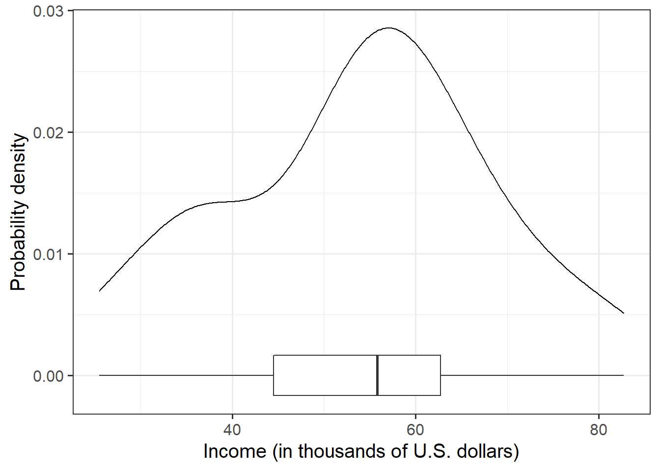
Display and describe the marginal distribution of employee incomes.

Solution

We can plot the marginal distribution of employee incomes as a density curve, and add a boxplot underneath to check for the presence of outliers.

Note: The function ggMarginal() from the ggExtra library only works with scatterplots.

ggplot(data = riverview, aes(x = income)) +
  geom_density() +
  geom_boxplot(width = 1/300) +
  labs(x = "Income (in thousands of U.S. dollars)", 
       y = "Probability density")

Figure 1: Density plot and boxplot of employee incomes.

The plot suggests that the distribution of employee incomes is unimodal and most of the incomes are between roughly $45,000 and $70,000. The smallest income in the sample is about $25,000 and the largest income is over $80,000. (We could find the exact values using the summary() function). This suggests there is a fair amount of variation in the data. Furthermore, the boxplot does not highlight any outliers in the data.

To further summarize the distribution, it is typical to compute and report numerical summary statistics such as the mean and standard deviation. One way to compute these values is to use the summary() function from the tidyverse library:

riverview %>% 
  summarize(
    M = mean(income), 
    SD = sd(income)
    )

## # A tibble: 1 x 2
##       M    SD
##   <dbl> <dbl>
## 1  53.7  14.6

Following the exploration above, we can describe this variable as follows:

The marginal distribution of income is unimodal with a mean of approximately $53,700. There is variation in employees’ salaries (SD = $14,553).

Question 3

Display and describe the marginal distribution of education level.

Solution

We can visualise the marginal distribution of education level using a density curve, and add a boxplot underneath to check for the presence of outliers.

ggplot(data = riverview, aes(x = education)) +
  geom_density() +
  geom_boxplot(width = 1/100) +
  labs(x = "Education (in years)", 
       y = "Probability density")

Figure 2: Density plot and boxplot of employee education levels.

Below are the summary statistics for the employees’ level of education:

riverview %>%
  summarize(
    M = mean(education),
    SD = sd(education)
    )

## # A tibble: 1 x 2
##       M    SD
##   <dbl> <dbl>
## 1    16  4.36

Again, we might write:

The marginal distribution of education is unimodal with a mean of 16 years. There is variation in employees’ level of education (SD = 4.4 years).

Relationship between variables

After examining the marginal distributions of the variables of interest in the analysis, we typically move on to examining relationships between the variables.

When describing the relationship between two numeric variables, we typically look at their scatterplot and comment on four characteristics of the relationship:

1. The direction of the association indicates whether large values of one variable tend to go with large values of the other (positive association) or with small values of the other (negative association).
2. The form of association refers to whether the relationship between the variables can be summarized well with a straight line or some more complicated pattern.
3. The strength of association entails how closely the points fall to a recognizable pattern such as a line.
4. Unusual observations that do not fit the pattern of the rest of the observations and which are worth examining in more detail.

Question 4

Create a scatterplot of income and education level.

Solution

We are trying to investigate how income varies when varying years of formal education. Hence income is the dependent variable (on the y-axis), and education is the independent variable (on the x-axis).

ggplot(data = riverview, aes(x = education, y = income)) +
  geom_point(alpha = 0.5) +
  labs(x = "Education (in years)", 
       y = "Income (in thousands of U.S. dollars)")

Figure 3: The relationship between employees’ education level and income.

Question 5

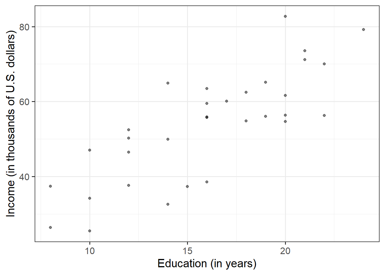
Use the scatterplot above to describe the relationship between income and level of education among the employees in the sample.

Solution

To comment on the strength of the linear association we compute the correlation coefficient:

riverview %>%
  select(education, income) %>%
  cor()

##           education    income
## education 1.0000000 0.7947847
## income    0.7947847 1.0000000

that is, \[ r_{\text{education, income}} = 0.79 \]

We might write:

There is a strong positive linear relationship between education level and income for the employees in the sample. High incomes tend to be observed, on average, with more years of formal education. The scatterplot does not highlight any outliers.

Model specification and fitting

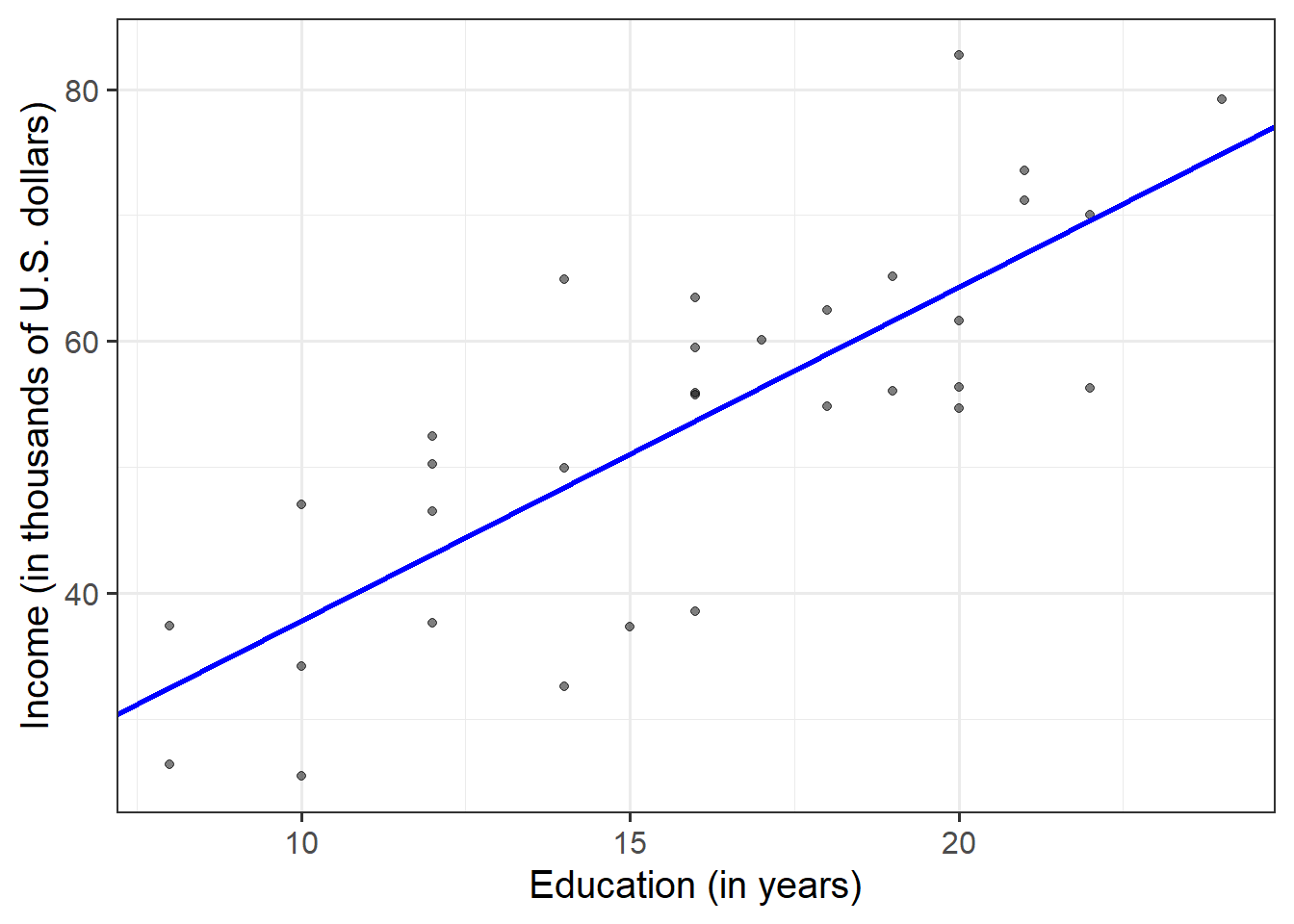
The scatterplot highlights a linear relationship, where the data points are scattered around an underlying linear pattern with a roughly-constant spread as x varies.

Hence, we will try to fit a simple (= one x variable only) linear regression model:

\[ y = \beta_0 + \beta_1 x + \epsilon \quad \text{where} \quad \epsilon \sim N(0, \sigma) \text{ independently} \]

where “\(\epsilon \sim N(0, \sigma) \text{ independently}\)” means that the errors around the line have mean zero and constant spread as x varies.

Question 6

Fit the linear model to the sample data using the lm() function and name the output mdl.

Write down the equation of the fitted line.

Hint: The syntax of the lm() function is:

lm(<response variable> ~ 1 + <explanatory variable>, data = <dataframe>)

Solution

The fitted model can be written as \[ \widehat{Income} = \hat \beta_0 + \hat \beta_1 \ Education \] or \[ \widehat{Income} = \hat \beta_0 \cdot 1 + \hat \beta_1 \cdot Education \]

When we specify the linear model in R, we include after the tilde sign, ~, the variables that appear to the right of the \(\hat \beta\)s. That’s why the 1 is included.

As the variables are in the riverview dataframe, we would write:

mdl <- lm(income ~ 1 + education, data = riverview)
mdl

## 
## Call:
## lm(formula = income ~ 1 + education, data = riverview)
## 
## Coefficients:
## (Intercept)    education  
##      11.321        2.651

Note that by calling the name of the fitted model, mdl, you can see the estimated regression coefficients \(\hat \beta_0\) and \(\hat \beta_1\). The fitted line is: \[ \widehat{Income} = 11.32 + 2.65 \ Education \\ \]

Question 7

Explore the following equivalent ways to obtain the estimated regression coefficients — that is, \(\hat \beta_0\) and \(\hat \beta_1\) — from the fitted model:

• mdl
• mdl$coefficients
• coef(mdl)
• coefficients(mdl)
• summary(mdl)

Solution

To obtain the estimated regression coefficients you can either:

• type mdl, i.e. simply invoke the name of the fitted model;
• type mdl$coefficients;
• use the coef(mdl) function;
• use the coefficients(mdl) function;
• use the summary(mdl) function and look under the “Estimate” column.

The estimated parameters returned by the above methods are all equivalent. However, summary() returns more information and you need to look under the column “Estimate.”

mdl

## 
## Call:
## lm(formula = income ~ 1 + education, data = riverview)
## 
## Coefficients:
## (Intercept)    education  
##      11.321        2.651

mdl$coefficients

## (Intercept)   education 
##   11.321379    2.651297

coef(mdl)

## (Intercept)   education 
##   11.321379    2.651297

coefficients(mdl)

## (Intercept)   education 
##   11.321379    2.651297

summary(mdl)

## 
## Call:
## lm(formula = income ~ 1 + education, data = riverview)
## 
## Residuals:
##     Min      1Q  Median      3Q     Max 
## -15.809  -5.783   2.088   5.127  18.379 
## 
## Coefficients:
##             Estimate Std. Error t value Pr(>|t|)    
## (Intercept)  11.3214     6.1232   1.849   0.0743 .  
## education     2.6513     0.3696   7.173 5.56e-08 ***
## ---
## Signif. codes:  0 '***' 0.001 '**' 0.01 '*' 0.05 '.' 0.1 ' ' 1
## 
## Residual standard error: 8.978 on 30 degrees of freedom
## Multiple R-squared:  0.6317, Adjusted R-squared:  0.6194 
## F-statistic: 51.45 on 1 and 30 DF,  p-value: 5.562e-08

The estimated intercept is \(\hat \beta_0 = 11.32\) and the estimated slope is \(\hat \beta_1 = 2.65\).

Question 8

Interpret the estimated intercept and slope in the context of the question of interest.

Solution

We can interpret the estimated intercept as follows,

The estimated average income associated to zero years of formal education is $11,321.

For the estimated slope we might write,

The estimated increase in average income associated to a one year increase in education is $2,651.

Question 9

Explore the following equivalent ways to obtain the estimated standard deviation of the errors — that is, \(\hat \sigma\) — from the fitted model mdl:

• sigma(mdl)
• summary(mdl)

Huh? What is \(\sigma\)?

The standard deviation of the errors, denoted by \(\sigma\) is an important quantity to estimate because it measures how much individual data points tend to deviate above and below the regression line.

A small \(\sigma\) indicates that the points hug the line closely and we should expect fairly accurate predictions, while a large \(\sigma\) suggests that, even if we estimate the line perfectly, we can expect individual values to deviate from it by substantial amounts.

The estimated standard deviation of the errors is (surprisingly) denoted \(\hat \sigma\) and is equal to \[ \hat \sigma = \sqrt{\frac{SS_{Residual}}{n - 2}} \]

Solution

The estimated standard deviation of the errors can be equivalently obtained by:

• typing sigma(mdl);
• looking at the “Residual standard error” entry of the summary(mdl) output.

Note: The term “Residual standard error” is a misnomer, as the help page for sigma says (check ?sigma). However, it’s hard to get rid of this bad name as it has been used in too many books showing R output.

sigma(mdl)

## [1] 8.978116

summary(mdl)

## 
## Call:
## lm(formula = income ~ 1 + education, data = riverview)
## 
## Residuals:
##     Min      1Q  Median      3Q     Max 
## -15.809  -5.783   2.088   5.127  18.379 
## 
## Coefficients:
##             Estimate Std. Error t value Pr(>|t|)    
## (Intercept)  11.3214     6.1232   1.849   0.0743 .  
## education     2.6513     0.3696   7.173 5.56e-08 ***
## ---
## Signif. codes:  0 '***' 0.001 '**' 0.01 '*' 0.05 '.' 0.1 ' ' 1
## 
## Residual standard error: 8.978 on 30 degrees of freedom
## Multiple R-squared:  0.6317, Adjusted R-squared:  0.6194 
## F-statistic: 51.45 on 1 and 30 DF,  p-value: 5.562e-08

The estimated standard deviation of the errors is \(\hat \sigma = 8.98\).

Question 10

Interpret the estimated standard deviation of the errors in the context of the research question.

Solution

To interpret the estimated standard deviation of the errors we can use the fact that about 95% of values from a normal distribution fall within two standard deviations of the centre.

For any particular level of education, employee incomes should be distributed above and below the regression line with standard deviation estimated to be \(\hat \sigma = 8.98\). Since \(2 \hat \sigma = 2 (8.98) = 17.96\), we expect most (about 95%) of the employee incomes to be within about $18,000 from the regression line.

Question 11

Plot the data and the fitted regression line. To do so:

• Extract the estimated regression coefficients e.g. via betas <- coef(mdl)
• Extract the first entry of betas via betas[1]
• Extract the second entry of betas via betas[2]
• Provide the intercept and slope to the function

geom_abline(intercept = <intercept>, slope = <slope>)

Solution

The function coef(mdl) returns a vector: that is, a sequence of numbers all of the same type. To get the first element of the sequence you append [1], and [2] for the second.

We can plot the model as follows:

betas <- coef(mdl)
intercept <- betas[1]
slope <- betas[2]

ggplot(data = riverview, aes(x = education, y = income)) +
  geom_point(alpha = 0.5) +
  geom_abline(intercept = intercept, slope = slope, 
              color = 'blue', size = 1) + 
  labs(x = "Education (in years)", 
       y = "Income (in thousands of U.S. dollars)")

Fitted and predicted values

To compute the model-predicted values for the data in the sample:

• predict(<fitted model>)
• fitted(<fitted model>)
• fitted.values(<fitted model>)
• mdl$fitted.values

predict(mdl)

##        1        2        3        4        5        6        7        8 
## 32.53175 32.53175 37.83435 37.83435 37.83435 43.13694 43.13694 43.13694 
##        9       10       11       12       13       14       15       16 
## 43.13694 48.43953 48.43953 48.43953 51.09083 53.74212 53.74212 53.74212 
##       17       18       19       20       21       22       23       24 
## 53.74212 53.74212 56.39342 59.04472 59.04472 61.69601 61.69601 64.34731 
##       25       26       27       28       29       30       31       32 
## 64.34731 64.34731 64.34731 66.99861 66.99861 69.64990 69.64990 74.95250

To compute model-predicted values for other data:

• predict(<fitted model>, newdata = <dataframe>)

We first need to remember that the model predicts income using the independent variable education. Hence, if we want predictions for new data, we first need to create a tibble with a column called education containing the years of education for which we want the prediction.

newdata <- tibble(education = c(11, 23))
newdata

## # A tibble: 2 x 1
##   education
##       <dbl>
## 1        11
## 2        23

Then we take newdata and add a new column called income_hat, computed as the prediction from the fitted mdl using the newdata above:

newdata <- newdata %>%
  mutate(
    income_hat = predict(mdl, newdata = newdata)
  )
newdata

## # A tibble: 2 x 2
##   education income_hat
##       <dbl>      <dbl>
## 1        11       40.5
## 2        23       72.3

Residuals

The residuals represent the deviations between the actual responses and the predicted responses and can be obtained either as

• mdl$residuals;
• resid(mdl);
• residuals(mdl);
• computing them as the difference between the response and the predicted response.

Question 12

Use predict(mdl) to compute the fitted values and residuals. Mutate the riverview dataframe to include the fitted values and residuals as extra columns.

Assign to the following symbols the corresponding numerical values:

• \(y_{3}\) = response variable for unit \(i = 3\) in the sample data
• \(\hat y_{3}\) = fitted value for the third unit
• \(\hat \epsilon_{5} = y_{5} - \hat y_{5}\) = the residual corresponding to the 5th unit.

Solution

riverview_fitted <- riverview %>%
  mutate(
    income_hat = predict(mdl),
    resid = income - income_hat
  )

head(riverview_fitted)

## # A tibble: 6 x 8
##   education income seniority gender  male party       income_hat  resid
##       <dbl>  <dbl>     <dbl> <chr>  <dbl> <chr>            <dbl>  <dbl>
## 1         8   37.4         7 male       1 Democrat          32.5   4.92
## 2         8   26.4         9 female     0 Independent       32.5  -6.10
## 3        10   47.0        14 male       1 Democrat          37.8   9.20
## 4        10   34.2        16 female     0 Independent       37.8  -3.65
## 5        10   25.5         1 female     0 Republican        37.8 -12.4 
## 6        12   46.5        11 female     0 Democrat          43.1   3.35

• \(y_{3}\) = 47.03
• \(\hat y_{3}\) = 37.83
• \(\hat \epsilon_{5} = y_{5} - \hat y_{5}\) = -12.36

Inference for regression coefficients

Consider again the output of the summary() function:

summary(mdl)

## 
## Call:
## lm(formula = income ~ 1 + education, data = riverview)
## 
## Residuals:
##     Min      1Q  Median      3Q     Max 
## -15.809  -5.783   2.088   5.127  18.379 
## 
## Coefficients:
##             Estimate Std. Error t value Pr(>|t|)    
## (Intercept)  11.3214     6.1232   1.849   0.0743 .  
## education     2.6513     0.3696   7.173 5.56e-08 ***
## ---
## Signif. codes:  0 '***' 0.001 '**' 0.01 '*' 0.05 '.' 0.1 ' ' 1
## 
## Residual standard error: 8.978 on 30 degrees of freedom
## Multiple R-squared:  0.6317, Adjusted R-squared:  0.6194 
## F-statistic: 51.45 on 1 and 30 DF,  p-value: 5.562e-08

To quantify the amount of uncertainty in each estimated coefficient that is due to sampling variability, we use the standard error (SE) of the coefficient. Recall that a standard error gives a numerical answer to the question of how variable a statistic will be because of random sampling.

The standard errors are found in the column “Std. Error.” That is, the SE of the intercept is 6.1232, and the SE of the slope corresponding to the education variable is 0.3696.

In this example the slope, 2.651, has a standard error of 0.37. One way to envision this is as a distribution. Our best guess (mean) for the slope parameter is 2.651. The standard deviation of this distribution is 0.37, which indicates the precision (uncertainty) of our estimate.

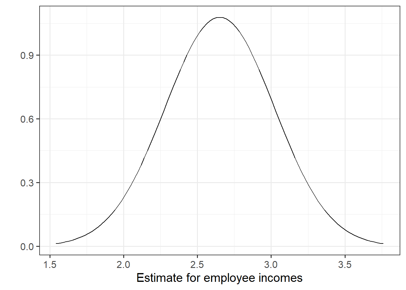
Figure 4: Sampling distribution of the slope coefficient. The distribution is approximately bell-shaped with a mean of 2.651 and a standard error of 0.37.

It shouldn’t surprise you that the reference distribution in this case is a t-distribution with \(n-2\) degrees of freedom, where \(n\) is the sample size. Recall the main formulas for obtaining a confidence interval and a test-statistic:

Test statistic

A test statistic for the null hypothesis \(H_0: \beta_1 = 0\) is \[ t = \frac{\hat \beta_1 - 0}{SE(\hat \beta_1)} \] which follows a t-distribution with \(n-2\) degrees of freedom.

Confidence interval

A confidence interval for the population slope is \[ \hat \beta_1 \pm t^* \cdot SE(\hat \beta_1) \] where \(t^*\) denotes the critical value chosen from t-distribution with \(n-2\) degrees of freedom for a desired \(\alpha\) level of confidence.

Question 13

Test the hypothesis that the population slope is zero — that is, that there is no linear association between income and education level in the population.

Solution

We calculate the test statistic \[ t = \frac{\hat \beta_1 - 0}{SE(\hat \beta_1)} = \frac{ 2.6513 - 0 }{0.3696} = 7.173 \] and compare it with the 5% critical value from a t-distribution with \(n-2\) degrees of freedom, which is:

n <- nrow(riverview)
tstar <- qt(0.975, df = n - 2)
tstar

## [1] 2.042272

As \(|t|\) is much larger than \(t^*\), we reject then null hypothesis as have strong evidence against it.

The p-value, shown below, also confirms the conclusion.

2 * (1 - pt(7.173, n - 2))

## [1] 5.561692e-08

Please note that the same information was already contained in the row corresponding to the variable “education” in the output of summary(mdl), which reported the t-statistic under t value and the p-value under Pr(>|t|):

summary(mdl)

## 
## Call:
## lm(formula = income ~ 1 + education, data = riverview)
## 
## Residuals:
##     Min      1Q  Median      3Q     Max 
## -15.809  -5.783   2.088   5.127  18.379 
## 
## Coefficients:
##             Estimate Std. Error t value Pr(>|t|)    
## (Intercept)  11.3214     6.1232   1.849   0.0743 .  
## education     2.6513     0.3696   7.173 5.56e-08 ***
## ---
## Signif. codes:  0 '***' 0.001 '**' 0.01 '*' 0.05 '.' 0.1 ' ' 1
## 
## Residual standard error: 8.978 on 30 degrees of freedom
## Multiple R-squared:  0.6317, Adjusted R-squared:  0.6194 
## F-statistic: 51.45 on 1 and 30 DF,  p-value: 5.562e-08

Before we interpret the results, recall that the p-value 5.56e-08 in the Pr(>|t|) column simply means \(5.56 \times 10^{-8}\). This is a very small value, hence we will report it as <.001 following the APA guidelines.

We performed a t-test against the null hypothesis that education is not a significant predictor of income: \(t(30) = 7.173,\ p < .001\), two-sided. The large t-statistic leads to a very small p-value, meaning that we have strong evidence against the null hypothesis.

Question 14

Compute a confidence interval for the regression slope

Solution

In the riverview example, for 95% confidence we have \(t^* = 2.04\):

n <- nrow(riverview)
tstar <- qt(0.975, df = n - 2)
tstar

## [1] 2.042272

The confidence interval is:

beta1_ci <- tibble(
  lower = 2.6513 - tstar * 0.3696,
  upper = 2.6513 + tstar * 0.3696,
)
beta1_ci

## # A tibble: 1 x 2
##   lower upper
##   <dbl> <dbl>
## 1  1.90  3.41

In R it is easy to obtain the confidence intervals for the regression coefficients using the command confint():

confint(mdl, level = 0.95)

##                 2.5 %    97.5 %
## (Intercept) -1.183935 23.826693
## education    1.896425  3.406168

The result is exactly the same (up to rounding errors) as the previous one.

We typically report our uncertainty in a statistic by providing \(\text{estimate} \pm t^* \cdot \text{SE}\). Here we would say that because of sampling variation, we are 95% confident that the slope is between 1.896 and 3.406. Interpreting this, we might say,

For all Riverview city employees, each one-year difference in formal education is associated with a difference in income between $1,896 and $3,406, on average.

Similarly, we could express the uncertainty in the intercept \(\hat \beta_0\) as:

The average income for all Riverview city employees with zero years of education is between $-1184 and $23,827.

References

Lewis-Beck, Colin, and Michael Lewis-Beck. 2015. Applied Regression: An Introduction. Vol. 22. Sage publications.