Two-way ANOVA
LEARNING OBJECTIVES
- Understand how to interpret interactions with effects coding.
- Understand how to interpret simple effects for experimental designs.
- Understand how to conduct pairwise comparisons.
Recap
You have (hopefully) already made a head start on this weeks exercises if you completed the Factorial ANOVA section of last week’s lab. If you haven’t yet completed these two questions, do so before reading any further.
In this week’s exercises, we will further explore questions such as:
- Does level \(i\) of the first factor have an effect on the response?
- Does level \(j\) of the second factor have an effect on the response?
- Is there a combined effect of level \(i\) of the first factor and level \(j\) of the second factor on the response? In other words, is there interaction of the two factors so that the combined effect is not simply the additive effect of level \(i\) of the first factor plus the effect of level \(j\) of the second factor?
Research question and data
As a reminder, we are working with data from a study yielding a \(3 \times 3\) factorial design to test whether there are differences in types of memory deficits for those experiencing different cognitive impairment(s).
| Diagnosis | grammar | classification | recognition |
|---|---|---|---|
| amnesic | 44, 63, 76, 72, 45 | 72, 66, 55, 82, 75 | 70, 51, 82, 66, 56 |
| huntingtons | 24, 30, 51, 55, 40 | 53, 59, 33, 37, 43 | 107, 80, 98, 82, 108 |
| control | 76, 98, 71, 70, 85 | 92, 65, 86, 67, 90 | 107, 80, 101, 82, 105 |
Interaction Model
Let’s look at the summary() and anova() output in detail from the model you should have previously fitted with the sum to zero constraint. As a reminder, the model with interaction is:
Applying the sum to zero constraint (for Diagnosis of ‘Control’ and Task of ‘Recognition’), we would have:
Based on previous plotting, it does seem that there is a clear interaction between diagnosis and task (as well as from our output above). However, we have not statistically compared our interaction model to an additive model (same model but without the interaction). Until we do so, we cannot confidently progress on the assumption that the interaction model is the most suitable for answering the research question.
We also want to consider the best coding constraint to apply in order to best answer the research question - are we interested in whether group X (e.g., Amnesic) differed from group Y (e.g., Huntingtons), or whether group X (e.g., Amnesic) differed from the overall group mean?
Since we are interested in comparing groups, we should reset to dummy coding, and thus should re-run our interaction model. Next, we need to perform a model comparison between the additive model and the interaction model using the anova() function.
After re-running your model with dummy coding, interpret the result of the model comparison.
\[\begin{aligned} Additive Model: Score &= \beta_0 \\ &+ \beta_1 D_\text{Amnseic} + \beta_2 D_\text{Huntingtons} \\ &+ \beta_3 T_\text{Grammar} + \beta_4 T_\text{Classification} \\ &+ \epsilon \end{aligned}\] \[\begin{aligned} Interaction Model: Score &= \beta_0 \\ &+ \beta_1 D_\text{Amnseic} + \beta_2 D_\text{Huntingtons} \\ &+ \beta_3 T_\text{Grammar} + \beta_4 T_\text{Classification} \\ &+ \beta_5 (D_\text{Amnseic} * T_\text{Grammar}) + \beta_6 (D_\text{Huntingtons} * T_\text{Grammar}) \\ &+ \beta_7 (D_\text{Amnseic} * T_\text{Classification}) + \beta_8 (D_\text{Huntingtons} * T_\text{Classification}) \\ &+ \epsilon \end{aligned}\]
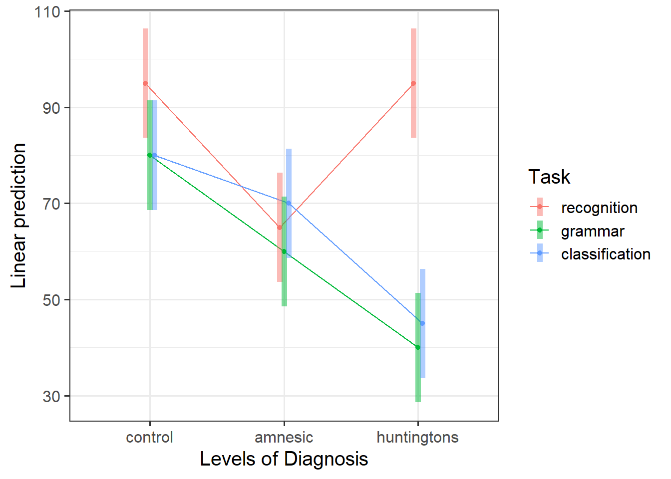
Using plot_model() (note that this function is from sjPlot package - make sure that you load this), generate a plot showing the predicted mean scores for each combination of levels of the diagnosis and task factors.

Contrast analysis
We will begin by looking at each factor separately.
In terms of the diagnostic groups, recall that we want to compare the amnesiacs to the Huntington individuals. This corresponds to a contrast with coefficients of 0, 1, and −1, for control, amnesic, and Huntingtons, respectively.
Similarly, in terms of the tasks, we want to compare the average of the two implicit memory tasks with the explicit memory task. This corresponds to a contrast with coefficients of 0.5, 0.5, and −1 for the three tasks.
When we are in presence of a significant interaction, the coefficients for a contrast between the means are found by multiplying each row coefficient with all column coefficients as shown below:

This can be done in R using:
diag_coef  <- c('control' = 0, 'amnesic' = 1, 'huntingtons' = -1)
task_coef  <- c('grammar' = 0.5, 'classification' = 0.5, 'recognition' = -1)
contr_coef <- outer(diag_coef, task_coef)   # or: diag_coef %o% task_coef
contr_coef
## grammar classification recognition
## control 0.0 0.0 0
## amnesic 0.5 0.5 -1
## huntingtons -0.5 -0.5 1The above coefficients correspond to testing the null hypothesis
\[ H_0 : \frac{\mu_{2,1} + \mu_{2,2}}{2} - \mu_{2,3} - \left( \frac{\mu_{3,1} + \mu_{3,2}}{2} - \mu_{3,3} \right) = 0 \]
or, equivalently,
\[ H_0 : \frac{\mu_{2,1} + \mu_{2,2}}{2} - \mu_{2,3} = \frac{\mu_{3,1} + \mu_{3,2}}{2} - \mu_{3,3} \]
which says that, in the population, the difference between the mean implicit memory and the explicit memory score is the same for amnesic patients and Huntingtons individuals. Note that the scores for the grammar and classification tasks have been averaged to obtain a single measure of ‘implicit memory’ score.
Now that we have the coefficients, let’s call the emmeans function (this is helpful to look at the ordering of the groups):
library(emmeans)
emm <- emmeans(mdl_int, ~ Diagnosis*Task)
emm
## Diagnosis Task emmean SE df lower.CL upper.CL
## control recognition 95 5.62 36 83.6 106.4
## amnesic recognition 65 5.62 36 53.6 76.4
## huntingtons recognition 95 5.62 36 83.6 106.4
## control grammar 80 5.62 36 68.6 91.4
## amnesic grammar 60 5.62 36 48.6 71.4
## huntingtons grammar 40 5.62 36 28.6 51.4
## control classification 80 5.62 36 68.6 91.4
## amnesic classification 70 5.62 36 58.6 81.4
## huntingtons classification 45 5.62 36 33.6 56.4
##
## Confidence level used: 0.95Next, from contr_coef, insert the coefficients following the order specified by the rows of emm above. That is, the first one should be for control recognition and have a value of 0, the second for amnesic recognition with a value of -1, and so on…
We also give a name to this contrast, such as ‘Research Hyp.’
comp_res <- contrast(emm, method = list('Research Hyp' = c(0, -1, 1, 0, 0.5, -0.5, 0, 0.5, -0.5)))
comp_res
## contrast estimate SE df t.ratio p.value
## Research Hyp 52.5 9.73 36 5.396 <.0001confint(comp_res)## contrast estimate SE df lower.CL upper.CL
## Research Hyp 52.5 9.73 36 32.8 72.2
##
## Confidence level used: 0.95or:
summary(comp_res, infer = TRUE)## contrast estimate SE df lower.CL upper.CL t.ratio p.value
## Research Hyp 52.5 9.73 36 32.8 72.2 5.396 <.0001
##
## Confidence level used: 0.95Interpret the results of the contrast analysis.
Simple Effects
By considering the simple effects, we can identify at which levels of the interacting condition we see different effects.
Since we have a significant interaction, we should also look at the simple main effects. Simple effects are the effect of one factor (e.g., Task) at each level of another factor (e.g., Diagnosis - Control, Huntingtons, and Amnesic).
Examine the simple effects for Task at each level of Diagnosis; and then the simple effects for Diagnosis at each level of Task.
There are various ways we can create an interaction plot, for instance, try this code:
emmip(mdl_int, Diagnosis ~ Task, CIs = TRUE)Considering the simple effects that we just saw in Question 5, identify the significant effects and match them to the parts of an interaction plot.

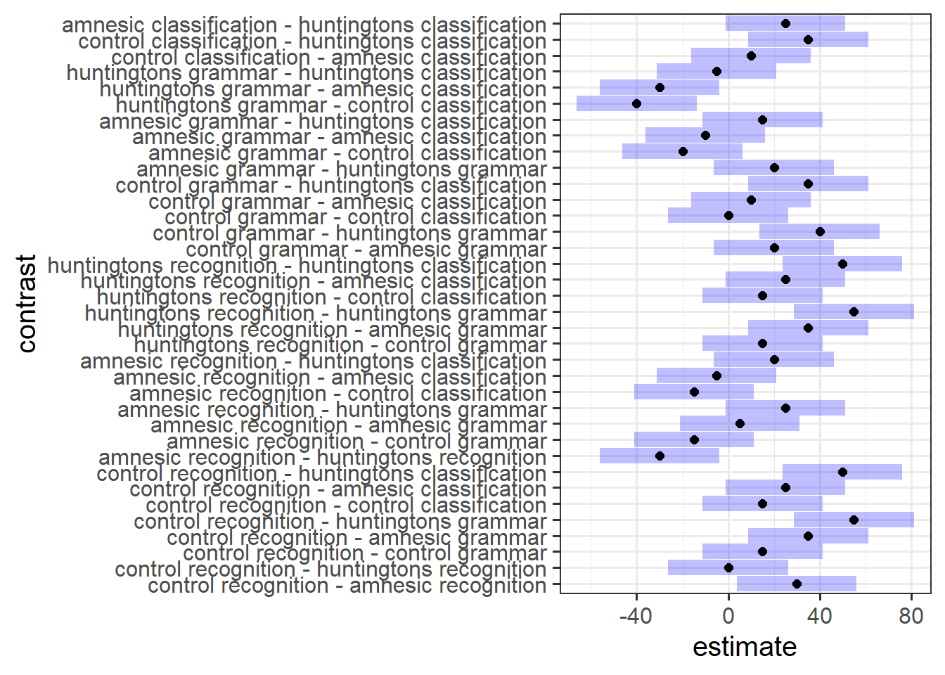
Pairwise Comparisons
Conduct exploratory pairwise comparisons to compare all levels of Diagnosis with all levels of Task.