Assumptions, Multiple Comparisons, Corrections, & Write-Up Example

LEARNING OBJECTIVES

1. Assess if a fitted model satisfies the assumptions of your model.
2. Understand how to apply corrections available for multiple comparisons.
   
3. Understand how to write-up and provide interpretation of a 2x2 factorial ANOVA.

Assumption Checks

With our cog data model, we have yet to check our assumptions (bad practice for us leaving it so late!). The good news is that most are the same as for linear regression. The only difference is that linearity is now replaced by checking whether the errors in each group have mean zero.

Question 1

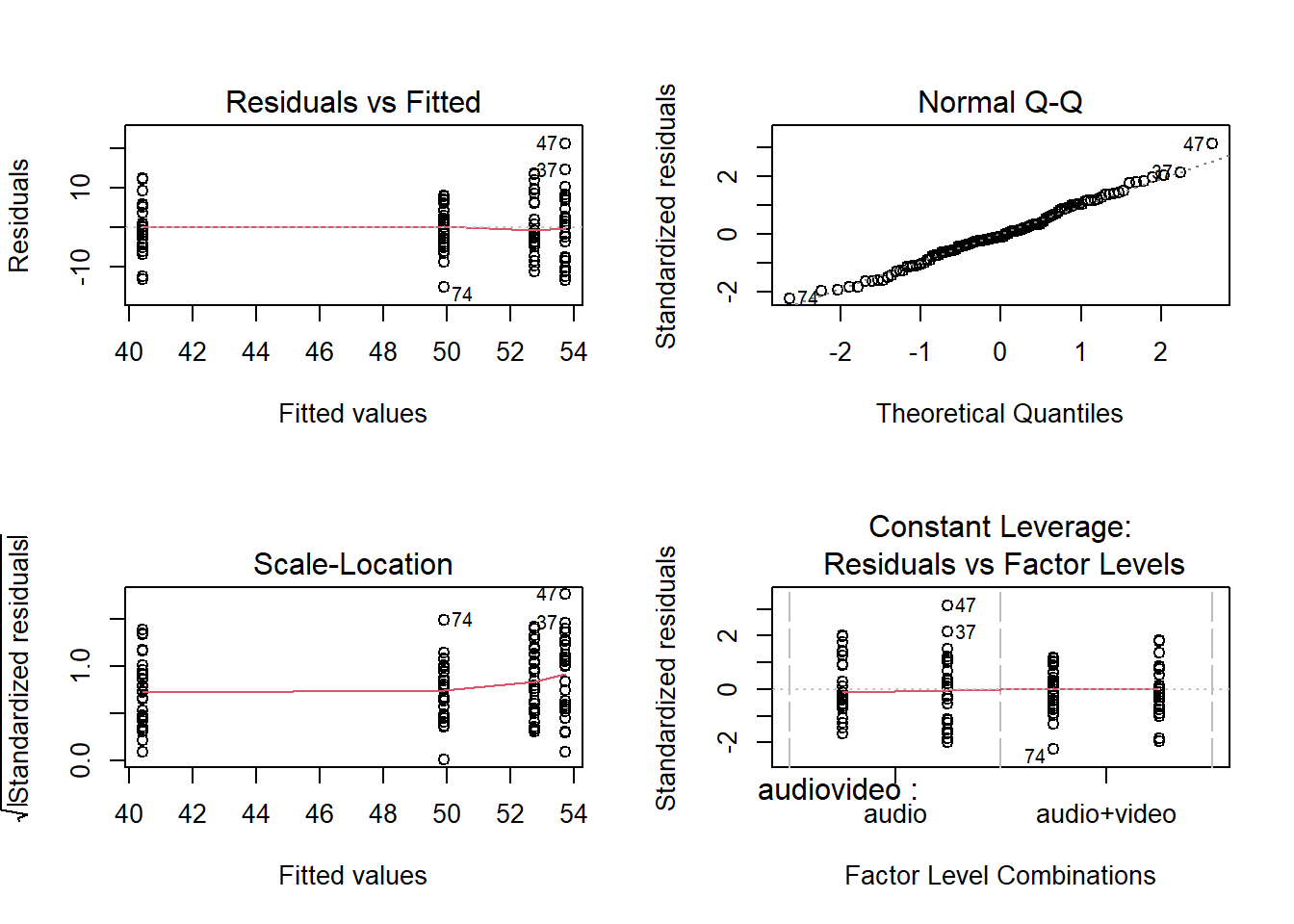
Let’s check that the interaction model doesn’t violate the assumptions.

• Are the errors independent?
• Do the errors have a mean of zero?
• Are the group variances equal?
• Is the distribution of the errors normal?

Solution

The plot of residuals vs fitted values shows that the residuals in each group are randomly scattered with a mean of zero. The scale location plots shows are fairly constant spread across the different groups.

The only concern is about normality of the errors. The qq-plot shows departures from the linear trend, and the histogram of the residuals isn’t bell-shaped.

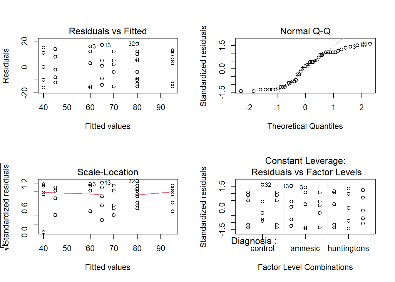
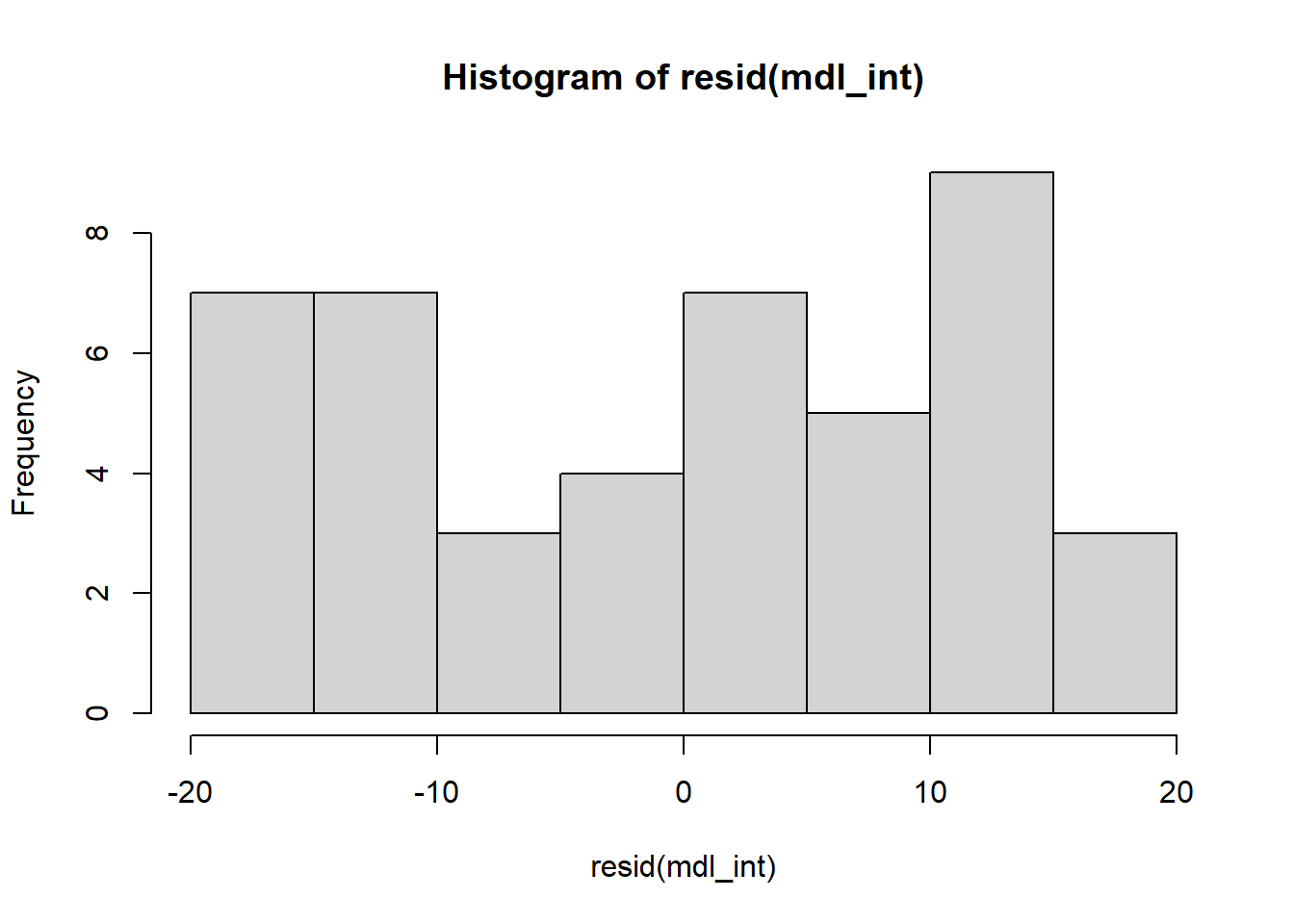
WARNING

The residuals don’t look like a sample from a normal population. For this reason, we can’t trust the model results and we should not generalise the results to the population as the hypothesis tests to be valid require all the assumptions to be met, including normality.

We will nevertheless carry on and finish this example so that we can exploring the remaining functions relevant for carrying out multiple comparisons with adjustments with a two-way ANOVA.

Multiple Comparisons

In last week’s exercises we began to look at how we compare different groups, by using contrast analysis to conduct tests of specific comparisons between groups. We also saw how we might conduct pairwise comparisons, where we test all possible pairs of group means within a given set.

For instance, we can compare the means of the different diagnosis groups for each task:

emm_task <- emmeans(mdl_int, ~ Diagnosis | Task)
contr_task <- contrast(emm_task, method = 'pairwise')
contr_task

## Task = recognition:
##  contrast              estimate   SE df t.ratio p.value
##  control - amnesic           30 7.94 36   3.776  0.0016
##  control - huntingtons        0 7.94 36   0.000  1.0000
##  amnesic - huntingtons      -30 7.94 36  -3.776  0.0016
## 
## Task = grammar:
##  contrast              estimate   SE df t.ratio p.value
##  control - amnesic           20 7.94 36   2.518  0.0424
##  control - huntingtons       40 7.94 36   5.035  <.0001
##  amnesic - huntingtons       20 7.94 36   2.518  0.0424
## 
## Task = classification:
##  contrast              estimate   SE df t.ratio p.value
##  control - amnesic           10 7.94 36   1.259  0.4273
##  control - huntingtons       35 7.94 36   4.406  0.0003
##  amnesic - huntingtons       25 7.94 36   3.147  0.0091
## 
## P value adjustment: tukey method for comparing a family of 3 estimates

or we can test all different combinations of task and diagnosis group (if that was something we were theoretically interested in, which is unlikely!) which would equate to conducting 36 comparisons!

emm_task <- emmeans(mdl_int, ~ Diagnosis * Task)
contr_task <- contrast(emm_task, method = 'pairwise')
contr_task

##  contrast                                             estimate   SE df t.ratio
##  control recognition - amnesic recognition                  30 7.94 36   3.776
##  control recognition - huntingtons recognition               0 7.94 36   0.000
##  control recognition - control grammar                      15 7.94 36   1.888
##  control recognition - amnesic grammar                      35 7.94 36   4.406
##  control recognition - huntingtons grammar                  55 7.94 36   6.923
##  control recognition - control classification               15 7.94 36   1.888
##  control recognition - amnesic classification               25 7.94 36   3.147
##  control recognition - huntingtons classification           50 7.94 36   6.294
##  amnesic recognition - huntingtons recognition             -30 7.94 36  -3.776
##  amnesic recognition - control grammar                     -15 7.94 36  -1.888
##  amnesic recognition - amnesic grammar                       5 7.94 36   0.629
##  amnesic recognition - huntingtons grammar                  25 7.94 36   3.147
##  amnesic recognition - control classification              -15 7.94 36  -1.888
##  amnesic recognition - amnesic classification               -5 7.94 36  -0.629
##  amnesic recognition - huntingtons classification           20 7.94 36   2.518
##  huntingtons recognition - control grammar                  15 7.94 36   1.888
##  huntingtons recognition - amnesic grammar                  35 7.94 36   4.406
##  huntingtons recognition - huntingtons grammar              55 7.94 36   6.923
##  huntingtons recognition - control classification           15 7.94 36   1.888
##  huntingtons recognition - amnesic classification           25 7.94 36   3.147
##  huntingtons recognition - huntingtons classification       50 7.94 36   6.294
##  control grammar - amnesic grammar                          20 7.94 36   2.518
##  control grammar - huntingtons grammar                      40 7.94 36   5.035
##  control grammar - control classification                    0 7.94 36   0.000
##  control grammar - amnesic classification                   10 7.94 36   1.259
##  control grammar - huntingtons classification               35 7.94 36   4.406
##  amnesic grammar - huntingtons grammar                      20 7.94 36   2.518
##  amnesic grammar - control classification                  -20 7.94 36  -2.518
##  amnesic grammar - amnesic classification                  -10 7.94 36  -1.259
##  amnesic grammar - huntingtons classification               15 7.94 36   1.888
##  huntingtons grammar - control classification              -40 7.94 36  -5.035
##  huntingtons grammar - amnesic classification              -30 7.94 36  -3.776
##  huntingtons grammar - huntingtons classification           -5 7.94 36  -0.629
##  control classification - amnesic classification            10 7.94 36   1.259
##  control classification - huntingtons classification        35 7.94 36   4.406
##  amnesic classification - huntingtons classification        25 7.94 36   3.147
##  p.value
##   0.0149
##   1.0000
##   0.6257
##   0.0026
##   <.0001
##   0.6257
##   0.0711
##   <.0001
##   0.0149
##   0.6257
##   0.9993
##   0.0711
##   0.6257
##   0.9993
##   0.2575
##   0.6257
##   0.0026
##   <.0001
##   0.6257
##   0.0711
##   <.0001
##   0.2575
##   0.0004
##   1.0000
##   0.9367
##   0.0026
##   0.2575
##   0.2575
##   0.9367
##   0.6257
##   0.0004
##   0.0149
##   0.9993
##   0.9367
##   0.0026
##   0.0711
## 
## P value adjustment: tukey method for comparing a family of 9 estimates

36? how do we know there are 36?

There are 3 diagnosis groups, and 3 tasks, meaning there are 9 different group means. All possible pairwise comparisons would is all different possible combinations of 2 from a set of 9. We can work this out using the rule:

\[ _nC_r = \frac{n!}{r!(n-r)!} \\ \begin{align} \\ & \text{Where:} \\ & n = \text{total number in the set} \\ & r = \text{number chosen} \\ & _nC_r = \text{number of combinations of r from n} \\ \end{align} \]

In R:

factorial(9)/(factorial(2)*(factorial(9-2)))

## [1] 36

Or, easier still:

dim(combn(9, 2))

## [1]  2 36

Why does the number of tests matter?

refresher on making errors in hypothesis tests

Think back to “Type 1 errors” from DAPR1 - when we conduct an hypothesis test, and we set \(\alpha=0.05\), we will reject the null hypothesis \(H_0\) when we find a \(p < .05\). Now remember what a \(p\)-value represents - it is the chance of observing a statistic at least as extreme as the one we do have, assuming the null hypothesis to be true. This means that if \(H_0\) is true, then we will still observe a \(p < .05\) 5% of the time. So our chance of making this error = the threshold (\(\alpha\)) at which below a p-value results in us rejecting \(H_0\).

But this error-rate applies to each statistical hypothesis we test. So if we conduct an experiment in which we plan on conducting lots of tests of different comparisons, the chance of an error being made increases substantially. Across the family of tests performed that chance will be much higher than 5%.¹

Each test conducted at \(\alpha = 0.05\) has a 0.05 (or 5%) probability of Type I error (wrongly rejecting the null hypothesis). If we do 9 tests, that experimentwise error rate is \(\alpha_{ew} \leq 9 \times 0.05\), where 9 is the number of comparisons made as part of the experiment.

Thus, if nine independent comparisons were made at the \(\alpha = 0.05\) level, the experimentwise Type I error rate \(\alpha_{ew}\) would be at most \(9 \times 0.05 = 0.45\). That is, we could wrongly reject the null hypothesis on average 45 times out of 100. To make this more confusing, many of the tests in a family are not independent (see the lecture slides for the calculation of error rate for dependent tests).

Here, we go through some of the different options available to us to control, or ‘correct’ for this problem.

Corrections

Bonferroni

Question 2

Load the data from last week, and re-acquaint yourself with it.

Provide a plot of the Diagnosis*Task group mean scores.

The data is at https://uoepsy.github.io/data/cognitive_experiment.csv.

Solution

cog <- read_csv('https://uoepsy.github.io/data/cognitive_experiment.csv')
# head(df)

cog$Diagnosis <- factor(cog$Diagnosis, 
                       labels = c("amnesic", "huntingtons", "control"),
                       ordered = FALSE)

cog$Task <- factor(cog$Task, 
                  labels = c("grammar", "classification", "recognition"), 
                  ordered = FALSE)

cog$Diagnosis <- fct_relevel(cog$Diagnosis, "control")
cog$Task <- fct_relevel(cog$Task, "recognition")

cog <- cog %>%
    rename(Score = Y)

Question 3

Fit the interaction model, using lm(). Pass your model to the anova() function, to remind yourself that there is a significant interaction present.

Solution

mdl_int <- lm(Score ~ Task*Diagnosis, data = cog)
anova(mdl_int)

## Analysis of Variance Table
## 
## Response: Score
##                Df Sum Sq Mean Sq F value    Pr(>F)    
## Task            2   5250 2625.00 16.6373  7.64e-06 ***
## Diagnosis       2   5250 2625.00 16.6373  7.64e-06 ***
## Task:Diagnosis  4   5000 1250.00  7.9225 0.0001092 ***
## Residuals      36   5680  157.78                      
## ---
## Signif. codes:  0 '***' 0.001 '**' 0.01 '*' 0.05 '.' 0.1 ' ' 1

Question 4

There are various ways to make nice tables in RMarkdown.
Some of the most well known are:

• The knitr package has kable()
  
• The pander package has pander()

Pick one (or find go googling and find a package you like the look of), install the package (if you don’t already have it), then try to create a nice pretty ANOVA table rather than the one given by anova(model).

Solution

library(knitr)
kable(anova(mdl_int))

	Df	Sum Sq	Mean Sq	F value	Pr(>F)
Task	2	5250	2625.0000	16.637324	0.0000076
Diagnosis	2	5250	2625.0000	16.637324	0.0000076
Task:Diagnosis	4	5000	1250.0000	7.922535	0.0001092
Residuals	36	5680	157.7778	NA	NA

library(pander)
pander(anova(mdl_int))

Analysis of Variance Table

	Df	Sum Sq	Mean Sq	F value	Pr(>F)
Task	2	5250	2625	16.64	7.64e-06
Diagnosis	2	5250	2625	16.64	7.64e-06
Task:Diagnosis	4	5000	1250	7.923	0.0001092
Residuals	36	5680	157.8	NA	NA

Question 5

As in the previous week’s exercises, let us suppose that we are specifically interested in comparisons of the mean score across the different diagnosis groups for a given task.

Edit the code below to obtain the pairwise comparisons of diagnosis groups for each task. Use the Bonferroni method to adjust for multiple comparisons, and then obtain confidence intervals.

library(emmeans)
emm_task <- emmeans(mdl_int, ? )
contr_task <- contrast(emm_task, method = ?, adjust = ? )

Solution

emm_task <- emmeans(mdl_int, ~ Diagnosis | Task)
contr_task <- contrast(emm_task, method = "pairwise", adjust="bonferroni")
contr_task

## Task = recognition:
##  contrast              estimate   SE df t.ratio p.value
##  control - amnesic           30 7.94 36   3.776  0.0017
##  control - huntingtons        0 7.94 36   0.000  1.0000
##  amnesic - huntingtons      -30 7.94 36  -3.776  0.0017
## 
## Task = grammar:
##  contrast              estimate   SE df t.ratio p.value
##  control - amnesic           20 7.94 36   2.518  0.0492
##  control - huntingtons       40 7.94 36   5.035  <.0001
##  amnesic - huntingtons       20 7.94 36   2.518  0.0492
## 
## Task = classification:
##  contrast              estimate   SE df t.ratio p.value
##  control - amnesic           10 7.94 36   1.259  0.6486
##  control - huntingtons       35 7.94 36   4.406  0.0003
##  amnesic - huntingtons       25 7.94 36   3.147  0.0099
## 
## P value adjustment: bonferroni method for 3 tests

confint(contr_task)

## Task = recognition:
##  contrast              estimate   SE df lower.CL upper.CL
##  control - amnesic           30 7.94 36  10.0517     49.9
##  control - huntingtons        0 7.94 36 -19.9483     19.9
##  amnesic - huntingtons      -30 7.94 36 -49.9483    -10.1
## 
## Task = grammar:
##  contrast              estimate   SE df lower.CL upper.CL
##  control - amnesic           20 7.94 36   0.0517     39.9
##  control - huntingtons       40 7.94 36  20.0517     59.9
##  amnesic - huntingtons       20 7.94 36   0.0517     39.9
## 
## Task = classification:
##  contrast              estimate   SE df lower.CL upper.CL
##  control - amnesic           10 7.94 36  -9.9483     29.9
##  control - huntingtons       35 7.94 36  15.0517     54.9
##  amnesic - huntingtons       25 7.94 36   5.0517     44.9
## 
## Confidence level used: 0.95 
## Conf-level adjustment: bonferroni method for 3 estimates

adjusting \(\alpha\), adjusting p

In the lecture we talked about adjusting the \(\alpha\) level (i.e., instead of determining significance at \(p < .05\), we might adjust and determine a result to be statistically significant if \(p < .005\), depending on how many tests are in our family of tests).

Note what the functions in R do is adjust the \(p\)-value, rather than the \(\alpha\). The Bonferroni method simply multiplies the ‘raw’ p-value by the number of the tests.

Question 6

In question 4 above, there are 9 tests being performed, but there are 3 in each ‘family’ (each Task).

Try changing your answer to question 4 to use adjust = "none", rather than "bonferroni", and confirm that the p-values are 1/3 of the size.

Solution

The first Bonferroni adjusted p-value is 0.0492.

0.0492/3

## [1] 0.0164

Let’s check that this is the raw p-value:

contrast(emm_task, method = "pairwise", adjust="none")

## Task = recognition:
##  contrast              estimate   SE df t.ratio p.value
##  control - amnesic           30 7.94 36   3.776  0.0006
##  control - huntingtons        0 7.94 36   0.000  1.0000
##  amnesic - huntingtons      -30 7.94 36  -3.776  0.0006
## 
## Task = grammar:
##  contrast              estimate   SE df t.ratio p.value
##  control - amnesic           20 7.94 36   2.518  0.0164
##  control - huntingtons       40 7.94 36   5.035  <.0001
##  amnesic - huntingtons       20 7.94 36   2.518  0.0164
## 
## Task = classification:
##  contrast              estimate   SE df t.ratio p.value
##  control - amnesic           10 7.94 36   1.259  0.2162
##  control - huntingtons       35 7.94 36   4.406  0.0001
##  amnesic - huntingtons       25 7.94 36   3.147  0.0033

Šídák

Question 7

The Sidak approach is slightly less conservative than the Bonferroni adjustment. Doing this with the emmeans package is easy, can you figure out how?

Hint: you just have to change the adjust argument in contrast() function.

Solution

contrast(emm_task, method = "pairwise", adjust = "sidak")

## Task = recognition:
##  contrast              estimate   SE df t.ratio p.value
##  control - amnesic           30 7.94 36   3.776  0.0017
##  control - huntingtons        0 7.94 36   0.000  1.0000
##  amnesic - huntingtons      -30 7.94 36  -3.776  0.0017
## 
## Task = grammar:
##  contrast              estimate   SE df t.ratio p.value
##  control - amnesic           20 7.94 36   2.518  0.0484
##  control - huntingtons       40 7.94 36   5.035  <.0001
##  amnesic - huntingtons       20 7.94 36   2.518  0.0484
## 
## Task = classification:
##  contrast              estimate   SE df t.ratio p.value
##  control - amnesic           10 7.94 36   1.259  0.5185
##  control - huntingtons       35 7.94 36   4.406  0.0003
##  amnesic - huntingtons       25 7.94 36   3.147  0.0099
## 
## P value adjustment: sidak method for 3 tests

Tukey

Question 8

Like with Šídák, in R we can easily change to Tukey. Conduct pairwise comparisons of the scores of different Diagnosis groups on different Task types (i.e., the interaction), and use the Tukey adjustment.

Solution

emm_task <- emmeans(mdl_int, ~ Diagnosis*Task)
contr_task <- contrast(emm_task, method = "pairwise", adjust="tukey")
contr_task

##  contrast                                             estimate   SE df t.ratio
##  control recognition - amnesic recognition                  30 7.94 36   3.776
##  control recognition - huntingtons recognition               0 7.94 36   0.000
##  control recognition - control grammar                      15 7.94 36   1.888
##  control recognition - amnesic grammar                      35 7.94 36   4.406
##  control recognition - huntingtons grammar                  55 7.94 36   6.923
##  control recognition - control classification               15 7.94 36   1.888
##  control recognition - amnesic classification               25 7.94 36   3.147
##  control recognition - huntingtons classification           50 7.94 36   6.294
##  amnesic recognition - huntingtons recognition             -30 7.94 36  -3.776
##  amnesic recognition - control grammar                     -15 7.94 36  -1.888
##  amnesic recognition - amnesic grammar                       5 7.94 36   0.629
##  amnesic recognition - huntingtons grammar                  25 7.94 36   3.147
##  amnesic recognition - control classification              -15 7.94 36  -1.888
##  amnesic recognition - amnesic classification               -5 7.94 36  -0.629
##  amnesic recognition - huntingtons classification           20 7.94 36   2.518
##  huntingtons recognition - control grammar                  15 7.94 36   1.888
##  huntingtons recognition - amnesic grammar                  35 7.94 36   4.406
##  huntingtons recognition - huntingtons grammar              55 7.94 36   6.923
##  huntingtons recognition - control classification           15 7.94 36   1.888
##  huntingtons recognition - amnesic classification           25 7.94 36   3.147
##  huntingtons recognition - huntingtons classification       50 7.94 36   6.294
##  control grammar - amnesic grammar                          20 7.94 36   2.518
##  control grammar - huntingtons grammar                      40 7.94 36   5.035
##  control grammar - control classification                    0 7.94 36   0.000
##  control grammar - amnesic classification                   10 7.94 36   1.259
##  control grammar - huntingtons classification               35 7.94 36   4.406
##  amnesic grammar - huntingtons grammar                      20 7.94 36   2.518
##  amnesic grammar - control classification                  -20 7.94 36  -2.518
##  amnesic grammar - amnesic classification                  -10 7.94 36  -1.259
##  amnesic grammar - huntingtons classification               15 7.94 36   1.888
##  huntingtons grammar - control classification              -40 7.94 36  -5.035
##  huntingtons grammar - amnesic classification              -30 7.94 36  -3.776
##  huntingtons grammar - huntingtons classification           -5 7.94 36  -0.629
##  control classification - amnesic classification            10 7.94 36   1.259
##  control classification - huntingtons classification        35 7.94 36   4.406
##  amnesic classification - huntingtons classification        25 7.94 36   3.147
##  p.value
##   0.0149
##   1.0000
##   0.6257
##   0.0026
##   <.0001
##   0.6257
##   0.0711
##   <.0001
##   0.0149
##   0.6257
##   0.9993
##   0.0711
##   0.6257
##   0.9993
##   0.2575
##   0.6257
##   0.0026
##   <.0001
##   0.6257
##   0.0711
##   <.0001
##   0.2575
##   0.0004
##   1.0000
##   0.9367
##   0.0026
##   0.2575
##   0.2575
##   0.9367
##   0.6257
##   0.0004
##   0.0149
##   0.9993
##   0.9367
##   0.0026
##   0.0711
## 
## P value adjustment: tukey method for comparing a family of 9 estimates

We can also use the following, which doesn’t require the emmeans package. You might see this when you look online for resources. The aov() function is fitting an ANOVA model, and then TukeyHSD() compares between Diagnosis group; between Task type; and between Diagnosis*Task.

Run the code below yourself to see the output.

TukeyHSD(aov(Score ~ Diagnosis * Task, data = cog))

Scheffe

Question 9

Run the same pairwise comparison as above, but this time with the Scheffe adjustment.

Solution

emm_task <- emmeans(mdl_int, ~ Diagnosis * Task)
contr_task <- contrast(emm_task, method = "pairwise", adjust="scheffe")
contr_task

##  contrast                                             estimate   SE df t.ratio
##  control recognition - amnesic recognition                  30 7.94 36   3.776
##  control recognition - huntingtons recognition               0 7.94 36   0.000
##  control recognition - control grammar                      15 7.94 36   1.888
##  control recognition - amnesic grammar                      35 7.94 36   4.406
##  control recognition - huntingtons grammar                  55 7.94 36   6.923
##  control recognition - control classification               15 7.94 36   1.888
##  control recognition - amnesic classification               25 7.94 36   3.147
##  control recognition - huntingtons classification           50 7.94 36   6.294
##  amnesic recognition - huntingtons recognition             -30 7.94 36  -3.776
##  amnesic recognition - control grammar                     -15 7.94 36  -1.888
##  amnesic recognition - amnesic grammar                       5 7.94 36   0.629
##  amnesic recognition - huntingtons grammar                  25 7.94 36   3.147
##  amnesic recognition - control classification              -15 7.94 36  -1.888
##  amnesic recognition - amnesic classification               -5 7.94 36  -0.629
##  amnesic recognition - huntingtons classification           20 7.94 36   2.518
##  huntingtons recognition - control grammar                  15 7.94 36   1.888
##  huntingtons recognition - amnesic grammar                  35 7.94 36   4.406
##  huntingtons recognition - huntingtons grammar              55 7.94 36   6.923
##  huntingtons recognition - control classification           15 7.94 36   1.888
##  huntingtons recognition - amnesic classification           25 7.94 36   3.147
##  huntingtons recognition - huntingtons classification       50 7.94 36   6.294
##  control grammar - amnesic grammar                          20 7.94 36   2.518
##  control grammar - huntingtons grammar                      40 7.94 36   5.035
##  control grammar - control classification                    0 7.94 36   0.000
##  control grammar - amnesic classification                   10 7.94 36   1.259
##  control grammar - huntingtons classification               35 7.94 36   4.406
##  amnesic grammar - huntingtons grammar                      20 7.94 36   2.518
##  amnesic grammar - control classification                  -20 7.94 36  -2.518
##  amnesic grammar - amnesic classification                  -10 7.94 36  -1.259
##  amnesic grammar - huntingtons classification               15 7.94 36   1.888
##  huntingtons grammar - control classification              -40 7.94 36  -5.035
##  huntingtons grammar - amnesic classification              -30 7.94 36  -3.776
##  huntingtons grammar - huntingtons classification           -5 7.94 36  -0.629
##  control classification - amnesic classification            10 7.94 36   1.259
##  control classification - huntingtons classification        35 7.94 36   4.406
##  amnesic classification - huntingtons classification        25 7.94 36   3.147
##  p.value
##   0.1131
##   1.0000
##   0.8852
##   0.0329
##   0.0001
##   0.8852
##   0.3060
##   0.0003
##   0.1131
##   0.8852
##   0.9999
##   0.3060
##   0.8852
##   0.9999
##   0.6128
##   0.8852
##   0.0329
##   0.0001
##   0.8852
##   0.3060
##   0.0003
##   0.6128
##   0.0080
##   1.0000
##   0.9894
##   0.0329
##   0.6128
##   0.6128
##   0.9894
##   0.8852
##   0.0080
##   0.1131
##   0.9999
##   0.9894
##   0.0329
##   0.3060
## 
## P value adjustment: scheffe method with rank 8

When to use Which Correction

Bonferroni

• Use Bonferroni’s method when you are interested in a small number of planned contrasts (or pairwise comparisons).
• Bonferroni’s method is to divide alpha by the number of tests/confidence intervals.
• Assumes that all comparisons are independent of one another.
  
• It sacrifices slightly more power than Tukey’s method (discussed below), but it can be applied to any set of contrasts or linear combinations (i.e., it is useful in more situations than Tukey).
• It is usually better than Tukey if we want to do a small number of planned comparisons.

Šídák

• (A bit) more powerful than the Bonferroni method.
• Assumes that all comparisons are independent of one another.
• Less common than Bonferroni method, largely because it is more difficult to calculate (not a problem now we have computers).

Tukey

• It specifies an exact family significance level for comparing all pairs of treatment means.
  
• Use Tukey’s method when you are interested in all (or most) pairwise comparisons of means.

Scheffe

• It is the most conservative (least powerful) of all tests.
• It controls the family alpha level for testing all possible contrasts.
• It should be used if you have not planned contrasts in advance.
• For testing pairs of treatment means it is too conservative (you should use Bonferroni or Šídák).

In R, you can easily change which correction you are using via the adjust = argument.

Lie Detection Experiment - Write Up Example

In this section of the lab, you will be presented with a research question, and tasked with writing up and presenting your analyses. Try to write three complete sections - Analysis Strategy, Results, and Discussion. Make sure to familiarise yourself with the data available in the codebook below. We will use the questions to go through the analysis step by step, before writing up. Please note that the lab includes short example write ups that may not be complete for every question you are asked. It is intended to give you a sense of the style. Think about the steps you need to complete in order to answer the research question, and the order in which you should complete these. Under the solutions are the code chunks used to complete the steps outlined, and the write up section examples follow at the end.

Lie detectors: Data Codebook

120 participants took part in a study in which they were presented with 100 recordings, and were tasked with guessing whether the speaker in each recording was lying or whether they were telling the truth.

Participants scored points every time they correctly identified a truth or a lie, and lost points whenever they mistook a lie for a truth (or vice versa). The maximum possible points to be scored was 100.

Half of the participants (60) were shown recordings in audio and video, the other half were presented with only the audio track.

Prior to taking part in the experiment, participants were given material to read for 10 minutes. Half of the participants in each condition (30 in the audio-only condition, and 30 in the audiovideo condition) were given instructional material used by the Police Force to train detectives to pick up on dishonesty during interrogations via various verbal and non-verbal cues. The remaining 30 participants in each condition were given a series of cartoon strips to read.

The data is available at https://uoepsy.github.io/data/lietraining.csv

Research Question

Do Police training materials and the mode of communication influence the accuracy of veracity judgements?

Question 1

Step 1 is always to read in the data, then to explore, check, describe, and visualise it.

• Load the data
• Examine the data
• Check coding of variables (ie., are categorical variables factors?)
• Produce a descriptives table for the variables of interest
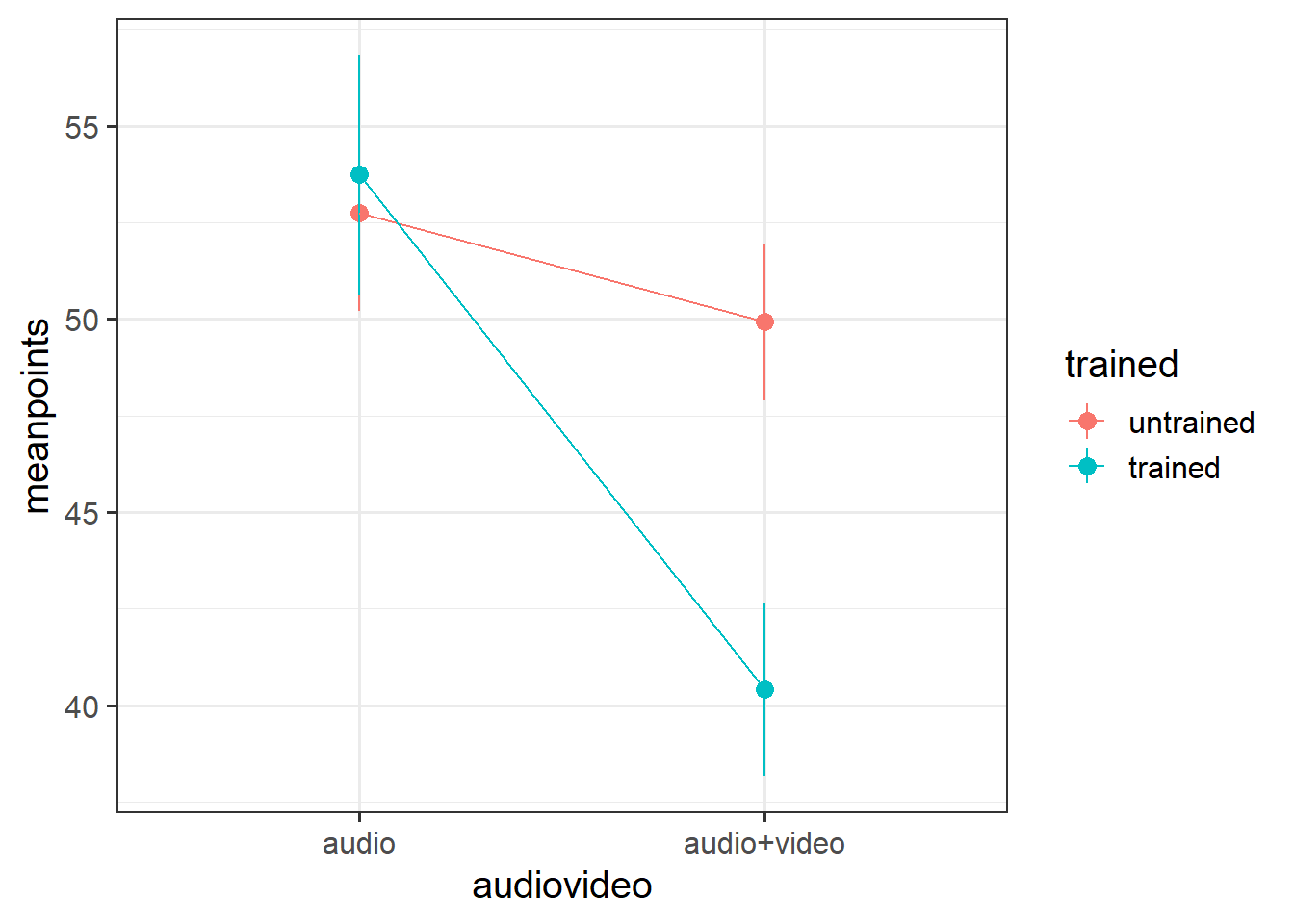
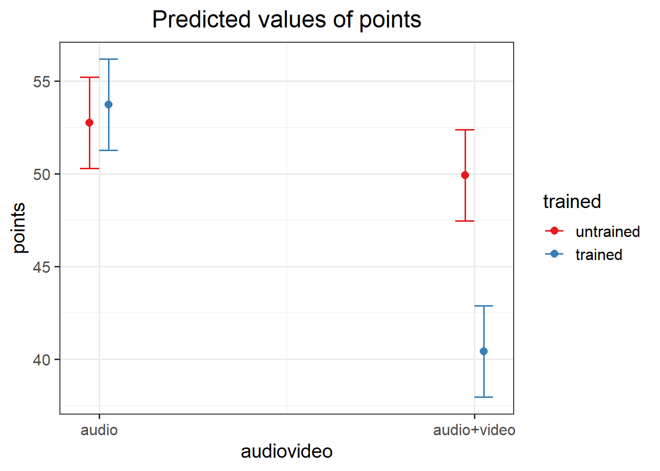
• Produce a plot showing the mean points for each condition

Solution

#read in data
liedat <- read_csv("https://uoepsy.github.io/data/lietraining.csv")

#check coding
head(liedat)

## # A tibble: 6 x 5
##   pid     age trained audiovideo  points
##   <chr> <dbl> <chr>   <chr>        <dbl>
## 1 ppt_1    26 y       audio+video   36.2
## 2 ppt_2    22 y       audio+video   38.5
## 3 ppt_3    18 y       audio+video   34.2
## 4 ppt_4    22 y       audio+video   52.6
## 5 ppt_5    21 y       audio+video   38.9
## 6 ppt_6    27 y       audio+video   37.5

#make variables factors & label
liedat$audiovideo <- factor(liedat$audiovideo, labels=c("audio","audio+video"))
liedat$trained <- factor(liedat$trained, labels = c("untrained","trained"))

#descriptives table
liestats <- liedat %>% group_by(audiovideo, trained) %>%
  summarise(meanpoints = mean(points),
            se = sd(points)/sqrt(n())
  )
liestats

## # A tibble: 4 x 4
## # Groups:   audiovideo [2]
##   audiovideo  trained   meanpoints    se
##   <fct>       <fct>          <dbl> <dbl>
## 1 audio       untrained       52.8  1.27
## 2 audio       trained         53.7  1.55
## 3 audio+video untrained       49.9  1.01
## 4 audio+video trained         40.4  1.12

#plot
ggplot(liestats, aes(x = audiovideo, y = meanpoints, color = trained)) + 
  geom_point(size = 3) +
  geom_linerange(aes(ymin = meanpoints - 2 * se, ymax = meanpoints + 2 * se)) +
  geom_path(aes(x = as.numeric(audiovideo)))

Question 2

Step 2 is to run your model(s) of interest to answer your research question, and make sure that the data meet the assumptions of your chosen test.

• Conduct a two-way ANOVA
• Check assumptions

Solution

#build model
lie_mdl <- lm(points ~ audiovideo * trained, data = liedat)

par(mfrow=c(2,2))
plot(lie_mdl)

par(mfrow=c(1,1))

# look at model output - summary() and anova()
summary(lie_mdl)

## 
## Call:
## lm(formula = points ~ audiovideo * trained, data = liedat)
## 
## Residuals:
##      Min       1Q   Median       3Q      Max 
## -15.1947  -4.2134  -0.7559   4.5235  21.1755 
## 
## Coefficients:
##                                      Estimate Std. Error t value Pr(>|t|)    
## (Intercept)                           52.7591     1.2576  41.953  < 2e-16 ***
## audiovideoaudio+video                 -2.8367     1.7785  -1.595    0.113    
## trainedtrained                         0.9759     1.7785   0.549    0.584    
## audiovideoaudio+video:trainedtrained -10.4830     2.5152  -4.168 5.95e-05 ***
## ---
## Signif. codes:  0 '***' 0.001 '**' 0.01 '*' 0.05 '.' 0.1 ' ' 1
## 
## Residual standard error: 6.888 on 116 degrees of freedom
## Multiple R-squared:  0.3768, Adjusted R-squared:  0.3607 
## F-statistic: 23.38 on 3 and 116 DF,  p-value: 6.591e-12

anova(lie_mdl)

## Analysis of Variance Table
## 
## Response: points
##                     Df Sum Sq Mean Sq F value    Pr(>F)    
## audiovideo           1 1957.7 1957.71  41.263 3.046e-09 ***
## trained              1  545.8  545.85  11.505   0.00095 ***
## audiovideo:trained   1  824.2  824.20  17.372 5.949e-05 ***
## Residuals          116 5503.6   47.45                      
## ---
## Signif. codes:  0 '***' 0.001 '**' 0.01 '*' 0.05 '.' 0.1 ' ' 1

Question 3

The third and final step(s) somewhat depends on the outcomes of step 2. Here, you may need to consider conducting further analyses before writing up / describing your results in relation to the research question.

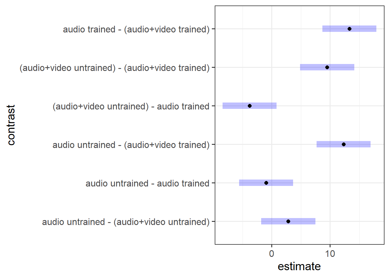
• Perform a pairwise comparison of the mean accuracy (as measured by points accrued) across the 2×2 factorial design, making sure to adjust for multiple comparisons by the method of your choice.
• Interpret your results in relation to the research question (remember you can refer to your previous plotting when doing this!).

Solution

emms_lie <- emmeans(lie_mdl, ~ audiovideo * trained)

lie_con <- contrast(emms_lie, method = "pairwise", adjust="tukey")
lie_con

##  contrast                                        estimate   SE  df t.ratio
##  audio untrained - (audio+video untrained)          2.837 1.78 116   1.595
##  audio untrained - audio trained                   -0.976 1.78 116  -0.549
##  audio untrained - (audio+video trained)           12.344 1.78 116   6.941
##  (audio+video untrained) - audio trained           -3.813 1.78 116  -2.144
##  (audio+video untrained) - (audio+video trained)    9.507 1.78 116   5.346
##  audio trained - (audio+video trained)             13.320 1.78 116   7.489
##  p.value
##   0.3855
##   0.9467
##   <.0001
##   0.1456
##   <.0001
##   <.0001
## 
## P value adjustment: tukey method for comparing a family of 4 estimates

# confidence intervals
confint(lie_con)

##  contrast                                        estimate   SE  df lower.CL
##  audio untrained - (audio+video untrained)          2.837 1.78 116    -1.80
##  audio untrained - audio trained                   -0.976 1.78 116    -5.61
##  audio untrained - (audio+video trained)           12.344 1.78 116     7.71
##  (audio+video untrained) - audio trained           -3.813 1.78 116    -8.45
##  (audio+video untrained) - (audio+video trained)    9.507 1.78 116     4.87
##  audio trained - (audio+video trained)             13.320 1.78 116     8.68
##  upper.CL
##     7.473
##     3.660
##    16.980
##     0.823
##    14.143
##    17.956
## 
## Confidence level used: 0.95 
## Conf-level adjustment: tukey method for comparing a family of 4 estimates

#plot
plot(lie_con)

Analysis Strategy

Example Write-Up of Analysis Strategy Section

Data obtained from https://uoepsy.github.io/data/lietraining.csv contained information on 120 participants who took part in a study concerning lie detection. Participants were each presented with 100 recordings (half were shown recordings in audio and video, and the other half audio only), and were tasked with guessing whether the speaker in each recording was lying or whether they were telling the truth. Participants scored 1 point each time they correctly identified a truth or a lie, and lost 1 point whenever they mistook a lie for a truth (or vice versa). The maximum score was 100, where higher scores reflected higher levels of accuracy. Prior to taking part in the experiment participants were given materials to read. Half of the participants in each condition were given instructional material used by the Police Force (used to train detectives to pick up on dishonesty during interrogations via various verbal and non-verbal cues) and the remaining 30 participants in each condition were given a series of cartoon strips to read.

All participant data was complete, and accuracy scores (points) within range i.e., 0-100. Categorical variables were coded as factors, where audio was the reference level for mode of communication, and untrained was the reference level for training materials.

To investigate whether police training materials (trained vs untrained) and the mode of communication (audio vs audiovideo) interacted to influence the accuracy of veracity judgements, a two-way ANOVA model was used. Effects were be considered statistically significant at \(\alpha = 0.05\). Using dummy coding, the following model specification was used:

\[\begin{aligned} \text{Points} &= \beta_0 \\ &+ \beta_1 A_\text{AudioVideo} + \beta_2 T_\text{Trained} \\ &+ \beta_3 (A_\text{AudioVideo} * T_\text{Trained}) \\ &+ \epsilon \end{aligned}\]

To address the research question of whether the interaction between training materials and mode of communication is significant, this corresponded to testing whether the interaction coefficient was equal to zero:

\[ H_0: \beta_3 = 0 \\ H_1: \beta_3 \neq 0 \]

The following assumptions were visually assessed using diagnostic plots: independence (with the previous plot and a plot of residuals vs index), equal variances (via a scale-location plot), and normality (via a qqplot of the residuals).

Results

Example Write-Up of Results Section

Descriptive statistics are displayed in Table 1.

Table 1: Descriptive Statistics

audiovideo	trained	meanpoints	se
audio	untrained	52.76	1.27
audio	trained	53.74	1.55
audio+video	untrained	49.92	1.01
audio+video	trained	40.42	1.12

In the audio condition, there did not appear to be a difference between trained and non-trained scores. However, untrained scored higher than trained in the audio+video condition. There appeared to be an interaction (see Figure 1).

Figure 1: Interaction Plot

Accuracy of veracity judgements (measured by points scored in lie-detecting game) were analysed with a 2 (audio vs audiovideo) \(\times\) 2 (untrained vs trained) between-subjects ANOVA.

Assumptions were visually assessed and met. The plot of residuals vs fitted values showed that the residuals in each group were randomly scattered with a mean of zero; the scale location plots showed a constant spread across the different groups; and the QQ-plot showed very little deviation from the diagonal line (see Figure 2).

Figure 2: Assumption Checks

There was a significant interaction between presentation mode and whether or not participants had received training for detecting lies \(F(1, 116) = 17.37, p <. 001\) (see Table ?? and Figure 3).

Analysis of Variance Table

	Df	Sum Sq	Mean Sq	F value	Pr(>F)
audiovideo	1	1958	1958	41.26	3.046e-09
trained	1	545.8	545.8	11.5	0.00095
audiovideo:trained	1	824.2	824.2	17.37	5.949e-05
Residuals	116	5504	47.45	NA	NA

Results suggested that the difference in points did not differ significantly in the audio condition regardless of training, but that there were significant differences in the audio video condition.

Figure 3: Predicted Scores

To explore the interaction further, pairwise comparisons were conducted. Tukey’s Honestly Significant Difference comparisons (see Figure 4) indicated that, contrary to what one might expect, participants who were presented with audiovisual recordings scored on average 9.5 points lower when they had read the police training materials compared to when they had received no training (95% CI [4.87 — 14.14]). The presentation mode (audio vs audio-video) was not found to result in a significantly different average score for those who were untrained (95% CI [-1.80 — 7.47]), and nor did training appear to have any effect on detecting lies in the audio-only condition (95% CI [-5.61 — 3.66]).

Figure 4: Tukey HSD Pairwise Comparisons

Discussion

Example Write-Up of Discussion Section

The findings indicated that, on the whole, people are bad at determining whether they are being presented with a lie or the truth, as the overall mean score was 49.2 out of 100 (SD = 8.61), where a series of completely random guesses expected to score 50/100. The police training materials did not appear to improve lie detection - trained participants performed more poorly (compared to untrained) in the audiovisual condition. This may indicate that the training materials focus too heavily on visual cues, which perhaps are not actually associated with dishonesty in the appropriate way.

---

1. what defines a ‘family’ of tests is debateable.↩︎