Information about solutions

Solutions for these exercises are available immediately below each question.
We would like to emphasise that much evidence suggests that testing enhances learning, and we strongly encourage you to make a concerted attempt at answering each question before looking at the solutions. Immediately looking at the solutions and then copying the code into your work will lead to poorer learning.
We would also like to note that there are always many different ways to achieve the same thing in R, and the solutions provided are simply one approach.

Be sure to check the solutions to last week’s exercises.
You can still ask any questions about previous weeks’ materials if things aren’t clear!

LEARNING OBJECTIVES

Understand the concept of an interaction.
Interpret the meaning of a numeric * categorical interaction.
Understand the principle of marginality and why this impacts modelling choices with interactions.
Visualize and probe interactions.

Exercises

Question 1

Reseachers have become interested in how the number of social interactions might influence mental health and wellbeing differently for those living in rural communities compared to those in cities and suburbs. They want to assess whether the effect of social interactions on wellbeing is moderated by (depends upon) whether or not a person lives in a rural area.

Create a new RMarkdown file, load the tidyverse package, and read in the wellbeing data into R.
The data is available at the following link: https://uoepsy.github.io/data/wellbeing.csv

Count the number of respondents in each location (City/Location/Rural).

Open-ended: Do you think there is enough data to answer this question?

Solution

library(tidyverse)
mwdata <- read_csv("https://uoepsy.github.io/data/wellbeing.csv")

mwdata %>% 
    count(location)

## # A tibble: 3 x 2
##   location     n
##   <chr>    <int>
## 1 City        15
## 2 Rural        7
## 3 Suburb      10

We have only 7 respondents who are from a rural location, and 25 from the city & suburbs. Intuitively, this doesn’t seem very many to rely on as representative of the population of those living in rural areas in Edinburgh & Lothians. Another thing to think about is that we probably don’t expect large differences between rural and city dwellers in the effect of social interaction on wellbeing (i.e., we might not expect differences in these sub-groups to be stronger than the overall relationship between social interaction and wellbeing).

Research Question: Does the relationship between number of social interactions and mental wellbeing differ between rural and non-rural residents?

To investigate how the relationship between the number of social interactions and mental wellbeing might be different for those living in rural communities, the researchers conduct a new study, collecting data from 200 randomly selected residents of the Edinburgh & Lothian postcodes.

Wellbeing/Rurality data codebook.

Download link

The data is available at https://uoepsy.github.io/data/wellbeing_rural.csv.

Description

From the Edinburgh & Lothians, 100 city/suburb residences and 100 rural residences were chosen at random and contacted to participate in the study. The Warwick-Edinburgh Mental Wellbeing Scale (WEMWBS), was used to measure mental health and well-being. Participants filled out a questionnaire including items concerning: estimated average number of hours spent outdoors each week, estimated average number of social interactions each week (whether on-line or in-person), whether a daily routine is followed (yes/no). For those respondents who had an activity tracker app or smart watch, they were asked to provide their average weekly number of steps.

The data in wellbeing_rural.csv contain seven attributes collected from a random sample of $n=200$ hypothetical residents over Edinburgh & Lothians, and include:

wellbeing: Warwick-Edinburgh Mental Wellbeing Scale (WEMWBS), a self-report measure of mental health and well-being. The scale is scored by summing responses to each item, with items answered on a 1 to 5 Likert scale. The minimum scale score is 14 and the maximum is 70.
outdoor_time: Self report estimated number of hours per week spent outdoors
social_int: Self report estimated number of social interactions per week (both online and in-person)
routine: Binary 1=Yes/0=No response to the question “Do you follow a daily routine throughout the week?”
location: Location of primary residence (City, Suburb, Rural)
steps_k: Average weekly number of steps in thousands (as given by activity tracker if available)
age: Age in years of respondent

Preview

The first six rows of the data are:

age	outdoor_time	social_int	routine	wellbeing	location	steps_k
28	12	13	1	36	rural	21.6
56	5	15	1	41	rural	12.3
25	19	11	1	35	rural	49.8
60	25	15	0	35	rural	NA
19	9	18	1	32	rural	48.1
34	18	13	1	34	rural	67.3

Question 2

Specify a multiple regression model to answer the research question.
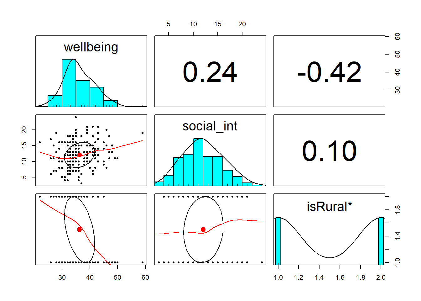
Read in the data, and assign it the name “mwdata2.” Then fully explore the variables and relationships which are going to be used in your analysis.

“Except in special circumstances, a model including a product term for interaction between two explanatory variables should also include terms with each of the explanatory variables individually, even though their coefficients may not be significantly different from zero. Following this rule avoids the logical inconsistency of saying that the effect of $X_1$ depends on the level of $X_2$ but that there is no effect of $X_1$.”
— Ramsey and Schafer (2012)

Tip 1: Install the psych package (remember to use the console, not your script to install packages), and then load it (load it in your script). The pairs.panels() function will plot all variables in a dataset against one another. This will save you the time you would have spent creating individual plots.
Tip 2: Check the “location” variable. It currently has three levels (Rural/Suburb/City), but we only want two (Rural/Not Rural). You’ll need to fix this. One way to do this would be to use ifelse() to define a variable which takes one value (“Rural”) if the observation meets from some condition, or another value (“Not Rural”) if it does not. Type ?ifelse in the console if you want to see the help function. You can use it to add a new variable either inside mutate(), or using data$new_variable_name <- ifelse(test, x, y) syntax.

Solution

To address the research question, we are going to fit the following model, where $y$ = wellbeing; $x_1$ = weekly outdoor time; and $x_2$ = whether or not the respondent lives in a rural location or not.

\[ y = \beta_0 + \beta_1 x_1 + \beta_2 x_2 + \beta_3 (x_1 \cdot x_2) + \epsilon \\ \quad \\ \text{where} \quad \epsilon \sim N(0, \sigma) \quad \text{independently} \]

First we read in the data, and take a quick look at our variables:

mwdata2 <- read_csv("https://uoepsy.github.io/data/wellbeing_rural.csv")
summary(mwdata2)

##       age         outdoor_time     social_int       routine        wellbeing   
##  Min.   :18.00   Min.   : 1.00   Min.   : 3.00   Min.   :0.000   Min.   :22.0  
##  1st Qu.:30.00   1st Qu.:12.75   1st Qu.: 9.00   1st Qu.:0.000   1st Qu.:33.0  
##  Median :42.00   Median :18.00   Median :12.00   Median :1.000   Median :35.0  
##  Mean   :42.30   Mean   :18.25   Mean   :12.06   Mean   :0.565   Mean   :36.3  
##  3rd Qu.:54.25   3rd Qu.:23.00   3rd Qu.:15.00   3rd Qu.:1.000   3rd Qu.:40.0  
##  Max.   :70.00   Max.   :35.00   Max.   :24.00   Max.   :1.000   Max.   :59.0  
##                                                                                
##    location            steps_k      
##  Length:200         Min.   :  0.00  
##  Class :character   1st Qu.: 24.00  
##  Mode  :character   Median : 42.45  
##                     Mean   : 44.93  
##                     3rd Qu.: 65.28  
##                     Max.   :111.30  
##                     NA's   :66

First let’s create a new variable for Rural/Not Rural

mwdata2 <- mwdata2 %>% 
  mutate(
    isRural = ifelse(location == "rural", "rural", "not rural")
  )

Now let’s use the pairs.panels() function from the psych package.
We could use it on the whole dataset, but for now we’ll just do it on the variables we’re interested in:

library(psych)

mwdata2 %>% 
  select(wellbeing, social_int, isRural) %>%
  pairs.panels()

Question 3

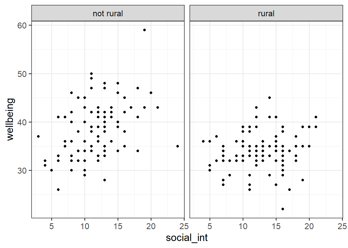
Produce a visualisation of the relationship between weekly number of social interactions and well-being, with separate facets for rural vs non-rural respondents.

Solution

Question 4

Fit your model using lm(), and assign it as an object with the name “rural_mod.”

Hint: When fitting a regression model in R with two explanatory variables A and B, and their interaction, these two are equivalent:

y ~ A + B + A:B
y ~ A*B

Solution

Interpreting coefficients for A and B in the presence of an interaction A:B

When you include an interaction between $x_1$ and $x_2$ in a regression model, you are estimating the extent to which the effect of $x_1$ on $y$ is different across the values of $x_2$.

What this means is that the effect of $x_1$ on $y$ depends on/is conditional upon the value of $x_2$.
(and vice versa, the effect of $x_2$ on $y$ is different across the values of $x_1$).
This means that we can no longer talk about the “effect of $x_1$ holding $x_2$ constant.” Instead we can talk about a marginal effect of $x_1$ on $y$ at a specific value of $x_2$.

When we fit the model $y = \beta_0 + \beta_1 x_1 + \beta_2 x_2 + \beta_3 (x_1 \cdot x_2) + \epsilon$ using lm():

the parameter estimate $\hat \beta_1$ is the marginal effect of $x_1$ on $y$ where $x_2 = 0$
the parameter estimate $\hat \beta_2$ is the marginal effect of $x_2$ on $y$ where $x_1 = 0$

N.B. Regardless of whether or not there is an interaction term in our model, all parameter estimates in multiple regression are “conditional” in the sense that they are dependent upon the inclusion of other variables in the model. For instance, in $y = \beta_0 + \beta_1 x_1 + \beta_2 x_2 + \epsilon$ the coefficient $\hat \beta_1$ is conditional upon holding $x_2$ constant.

Interpreting the interaction term A:B

The coefficient for an interaction term can be thought of as providing an adjustment to the slope.

In the model below, we have a numeric*categorical interaction: \[ \begin{align} \text{wellbeing} \ = \ &\beta_0 + \beta_1 \text{social_interactions} + \beta_2 \text{isRural} + \\ &\beta_3 (\text{social_interactions} \cdot \text{isRural}) + \epsilon \end{align} \]

The estimate $\hat \beta_3$ is the adjustment to the slope $\hat \beta_1$ to be made for the individuals in the $\text{isRural}=1$ group.

Question 5

Look at the parameter estimates from your model, and write a description of what each one corresponds to on the plot shown in Figure 1 (it may help to sketch out the plot yourself and annotate it).

“The best method of communicating findings about the presence of significant interaction may be to present a table of graph of the estimated means at various combinations of the interacting variables.”
— Ramsey and Schafer (2012)

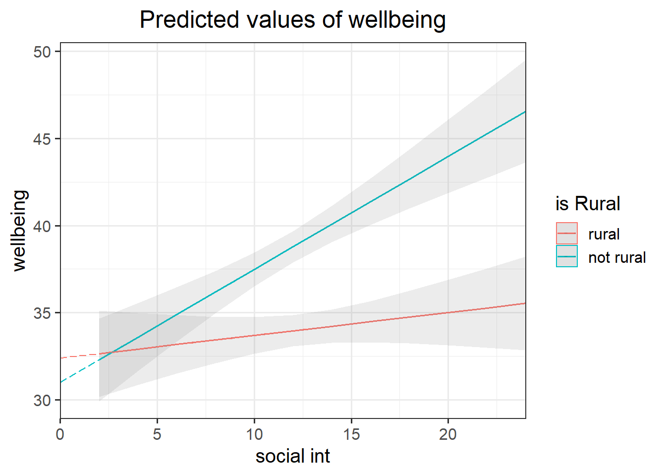
Multiple regression model: Wellbeing ~ Social Interactions * is Rural<br><small>Note that the dashed lines represent predicted values below the minimum observed number of social interactions, to ensure that zero on the x-axis is visible</small>

Figure 1: Multiple regression model: Wellbeing ~ Social Interactions * is Rural
Note that the dashed lines represent predicted values below the minimum observed number of social interactions, to ensure that zero on the x-axis is visible

Hints.

Solution

We can obtain our parameter estimates using various functions such as summary(rural_mod),coef(rural_mod), coefficients(rural_mod) etc.

coefficients(rural_mod)

##             (Intercept)              social_int            isRuralrural 
##              30.9985688               0.6487945               1.3865688 
## social_int:isRuralrural 
##              -0.5175856

$\hat \beta_0$ = (Intercept) = 31: The point at which the blue line cuts the y-axis (where social_int = 0).
$\hat \beta_1$ = social_int = 0.65: The slope (vertical increase on the y-axis associated with a 1 unit increase on the x-axis) of the blue line.
$\hat \beta_2$ = isRuralrural = 1.39: The vertical distance from the blue to the red line at the y-axis (where social_int = 0).
$\hat \beta_3$ = social_int:isRuralrural = -0.52: How the slope of the line changes when you move from the blue to the red line.

Question 6

Load the sjPlot package and try using the function plot_model().
The default behaviour of plot_model() is to plot the parameter estimates and their confidence intervals. This is where type = "est". Try to create a plot like Figure 1, which shows the two lines (Hint: what are this weeks’ exercises all about? type = ???.)

Solution

References

Ramsey, Fred, and Daniel Schafer. 2012. The Statistical Sleuth: A Course in Methods of Data Analysis. Cengage Learning.

Interactions: Numeric * Categorical

Exercises

References