Exercises
Question 1
Previous research has identified an association between an individual’s perception of their social rank and symptoms of depression, anxiety and stress. We are interested in the individual differences in this relationship.
Create a new RMarkdown, load the tidyverse package, read the social comparison study data into R and assign it the name “scs_study.” The data is available at https://uoepsy.github.io/data/scs_study.csv
Solution
library(tidyverse)
scs_study <- read_csv("https://uoepsy.github.io/data/scs_study.csv")
Research question
Does the effect of social comparison on symptoms of depression, anxiety and stress vary depending on level of neuroticism?
To investigate whether the effect of social comparison on symptoms of depression, anxiety and stress varies depending on level of neuroticism, we will need to fit a multiple regression model with an interaction term. Before we think about fitting our model, it is important that we understand the data available - how many participants? What type (or class) of data will we be working with? What was the measurement scale? How were scales scored? Look at the social comparison study data codebook below.
Social Comparison Study data codebook
Download link
The data is available to download at https://uoepsy.github.io/data/scs_study.csv
Description
Data from 656 participants containing information on scores on each trait of a Big 5 personality measure, their perception of their own social rank, and their scores on a measure of depression.
The data in scs_study.csv contain seven attributes collected from a random sample of \(n=656\) participants:
zo: Openness (Z-scored), measured on the Big-5 Aspects Scale (BFAS)zc: Conscientiousness (Z-scored), measured on the Big-5 Aspects Scale (BFAS)ze: Extraversion (Z-scored), measured on the Big-5 Aspects Scale (BFAS)za: Agreeableness (Z-scored), measured on the Big-5 Aspects Scale (BFAS)zn: Neuroticism (Z-scored), measured on the Big-5 Aspects Scale (BFAS)scs: Social Comparison Scale - An 11-item scale that measures an individual’s perception of their social rank, attractiveness and belonging relative to others. The scale is scored as a sum of the 11 items (each measured on a 5-point scale), with higher scores indicating more favourable perceptions of social rank.dass: Depression Anxiety and Stress Scale - The DASS-21 includes 21 items, each measured on a 4-point scale. The score is derived from the sum of all 21 items, with higher scores indicating higher a severity of symptoms.
Preview
The first six rows of the data are:
| zo |
zc |
ze |
za |
zn |
scs |
dass |
| 0.7587304 |
1.5838564 |
-0.79153841 |
-0.09104726 |
1.32023703 |
30 |
56 |
| 0.3033394 |
-0.2698774 |
-0.08636742 |
0.08849465 |
-0.40280445 |
30 |
48 |
| -0.1347251 |
0.6566343 |
-0.79796588 |
-0.94759192 |
0.92927138 |
35 |
48 |
| 1.0640775 |
-1.0218540 |
-0.16475623 |
-0.50409122 |
-0.02021664 |
29 |
48 |
| 1.7411706 |
-0.7773205 |
-1.55003059 |
-2.86050116 |
-1.14145028 |
41 |
43 |
| 0.2203023 |
-0.4054477 |
0.78397367 |
0.90388509 |
-0.24641819 |
37 |
60 |
Refresher: Z-scores
When we standardise a variable, we re-express each value as the distance from the mean in units of standard deviations. These transformed values are called z-scores.
To transform a given value \(x_i\) into a z-score \(z_i\), we simply calculate the distance from \(x_i\) to the mean, \(\bar{x}\), and divide this by the standard deviation, \(s\):
\[
z_i = \frac{x_i - \bar{x}}{s}
\]
A Z-score of a value is the number of standard deviations below/above the mean that the value falls.
Question 2
Specify the model you plan to fit in order to answer the research question (e.g., \(\text{??} = \beta_0 + \beta_1 \cdot \text{??} + .... + \epsilon\))
Solution
\[
\text{DASS-21 Score} = \beta_0 + \beta_1 \cdot \text{SCS Score} + \beta_2 \cdot \text{Neuroticism} + \beta_3 \cdot (\text{SCS score} \cdot \text{Neuroticism}) + \epsilon
\]
Question 3
Produce plots of the relevant distributions and relationships involved in the analysis.
Solution
ggplot(data = scs_study, aes(x=dass)) +
  geom_density() +
  geom_boxplot(width = 1/50) +
  labs(title="Marginal distribution of DASS-21 Scores",
       x = "Depression Anxiety and Stress Scale", y = "Probability density")
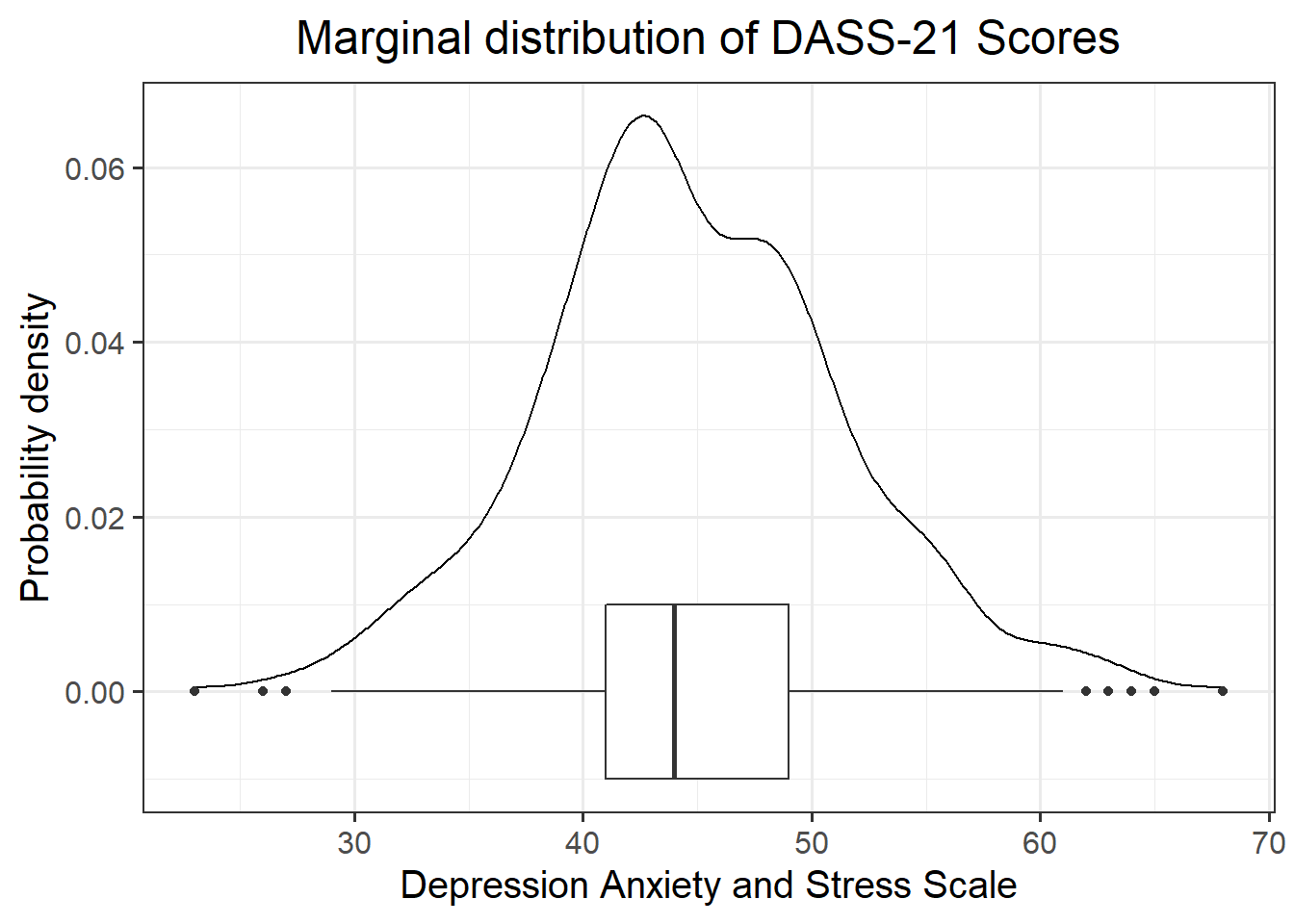
The marginal distribution of scores on the Depression, Anxiety and Stress Scale (DASS-21) is unimodal with a mean of approximately 45 and a standard deviation of 7.
ggplot(data = scs_study, aes(x=scs)) +
  geom_density() +
  geom_boxplot(width = 1/50) +
  labs(title="Marginal distribution of Social Comparison Scale (SCS) scores",
       x = "Social Comparison Scale Score", y = "Probability density")
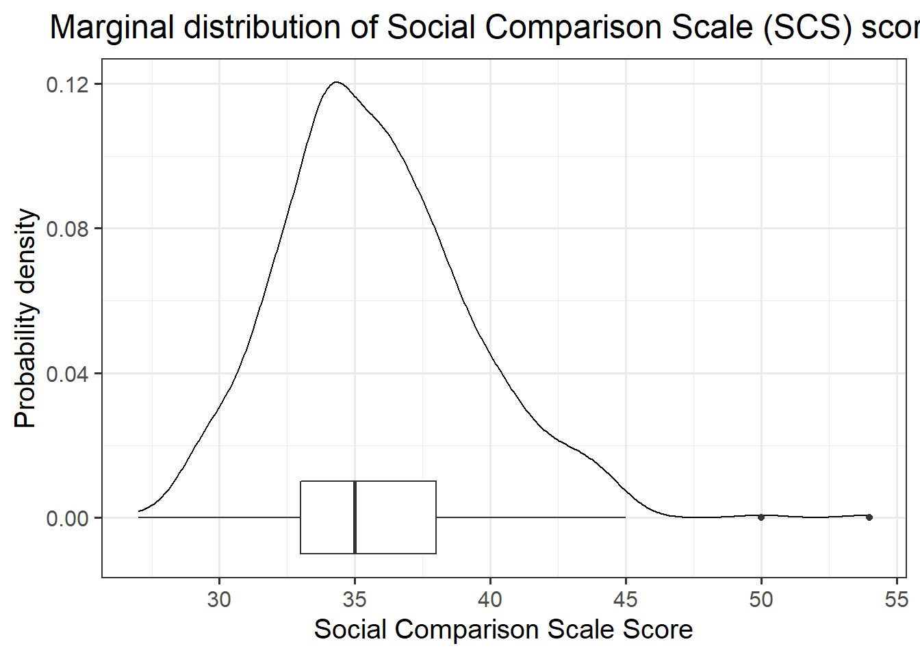
The marginal distribution of score on the Social Comparison Scale (SCS) is unimodal with a mean of approximately 36 and a standard deviation of 4. There look to be a number of outliers at the upper end of the scale.
ggplot(data = scs_study, aes(x=zn)) +
  geom_density() +
  geom_boxplot(width = 1/50) +
  labs(title="Marginal distribution of Neuroticism (Z-Scored)",
       x = "Neuroticism (Z-Scored)", y = "Probability density")
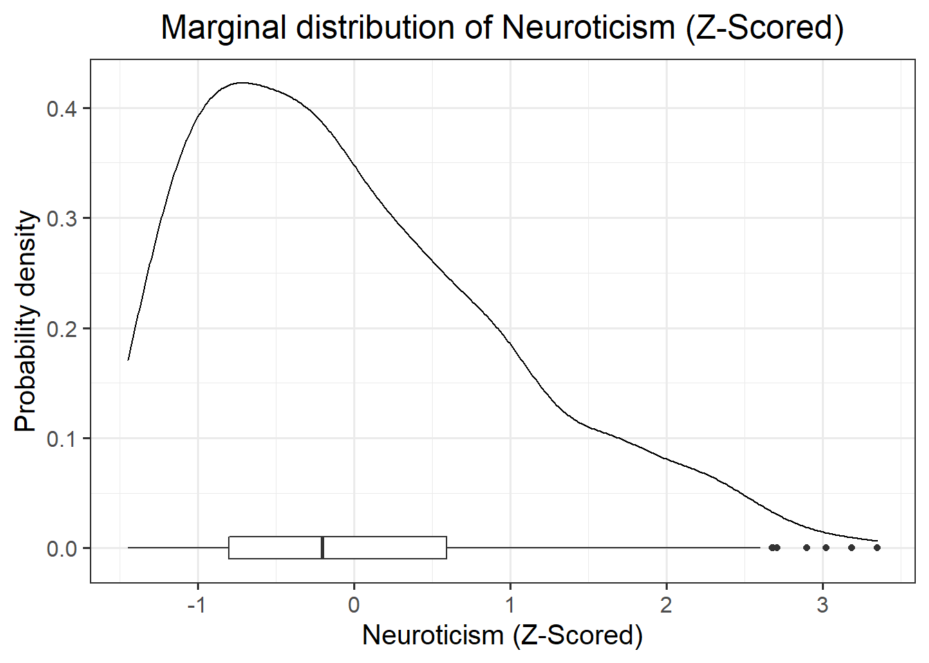
The marginal distribution of Neuroticism (Z-scored) is positively skewed, with the 25% of scores falling below -0.8, 75% of scores falling below 0.59.
library(patchwork) # for arranging plots side by side
library(kableExtra) # for making tables look nice
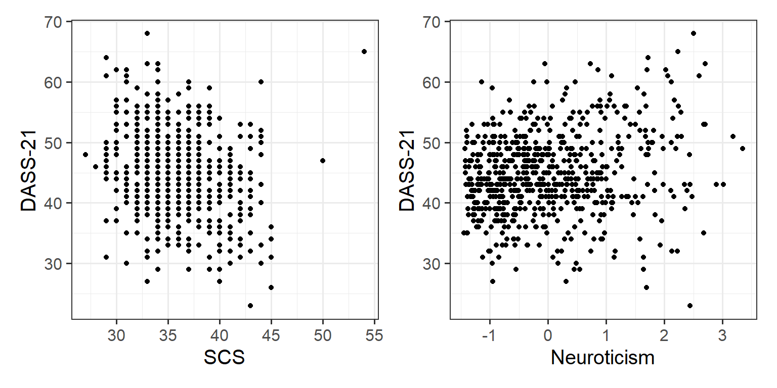
p1 <- ggplot(data = scs_study, aes(x=scs, y=dass)) +
geom_point()+
labs(x = "SCS", y = "DASS-21")
p2 <- ggplot(data = scs_study, aes(x=zn, y=dass)) +
geom_point()+
labs(x = "Neuroticism", y = "DASS-21")
p1 | p2
# the kable() function from the kableExtra package can make table outputs print nicely into html.
scs_study %>%
  select(dass, scs, zn) %>%
  cor() %>%
  kable(digits = 2) %>%
  kable_styling(full_width = FALSE)
|
|
dass
|
scs
|
zn
|
|
dass
|
1.00
|
-0.23
|
0.20
|
|
scs
|
-0.23
|
1.00
|
0.11
|
|
zn
|
0.20
|
0.11
|
1.00
|
There is a weak, negative, linear relationship between scores on the Social Comparison Scale and scores on the Depression Anxiety and Stress Scale for the participants in the sample. Severity of symptoms measured on the DASS-21 tend to decrease, on average, the more favourably participants view their social rank.
There is a weak, positive, linear relationship between the levels of Neuroticism and scores on the DASS-21. Participants who are more neurotic tend to, on average, display a higher severity of symptoms of depression, anxiety and stress.
Question 4
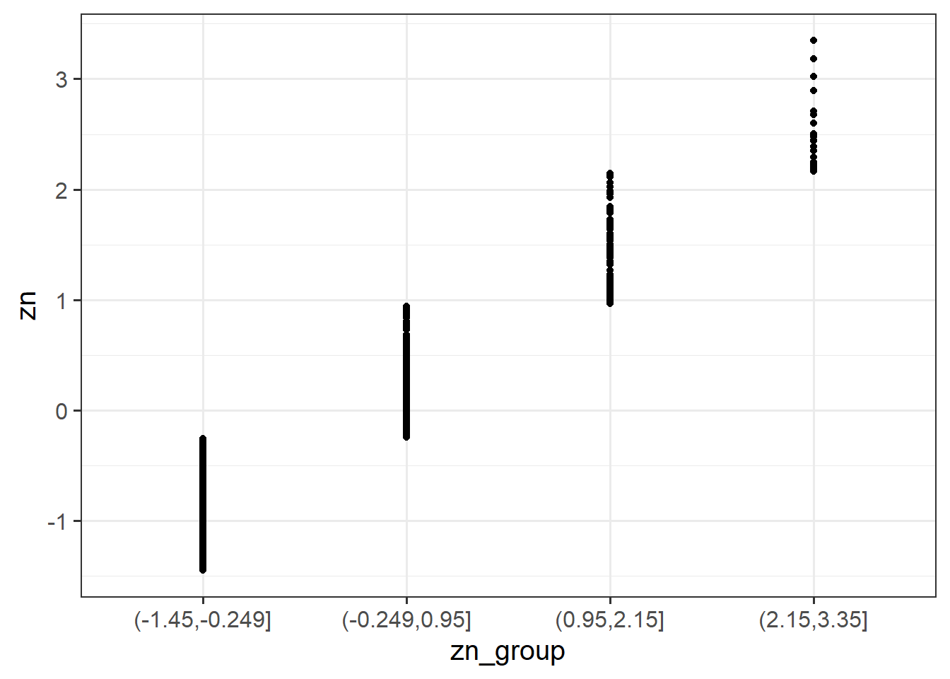
Run the code below. It takes the dataset, and uses the cut() function to add a new variable called “zn_group,” which is the “zn” variable split into 4 groups.
Remember: we have re-assign this output as the name of the dataset (the scs_study <- bit at the beginning) to make these changes occur in our environment (the top-right window of Rstudio). If we didn’t have the first line, then it would simply print the output.
scs_study <-
  scs_study %>%
  mutate(
    zn_group = cut(zn, 4)
  )
We can see how it has split the “zn” variable by plotting the two against one another:
(Note that the levels of the new variable are named according to the cut-points).
ggplot(data = scs_study, aes(x = zn_group, y = zn)) +
  geom_point()
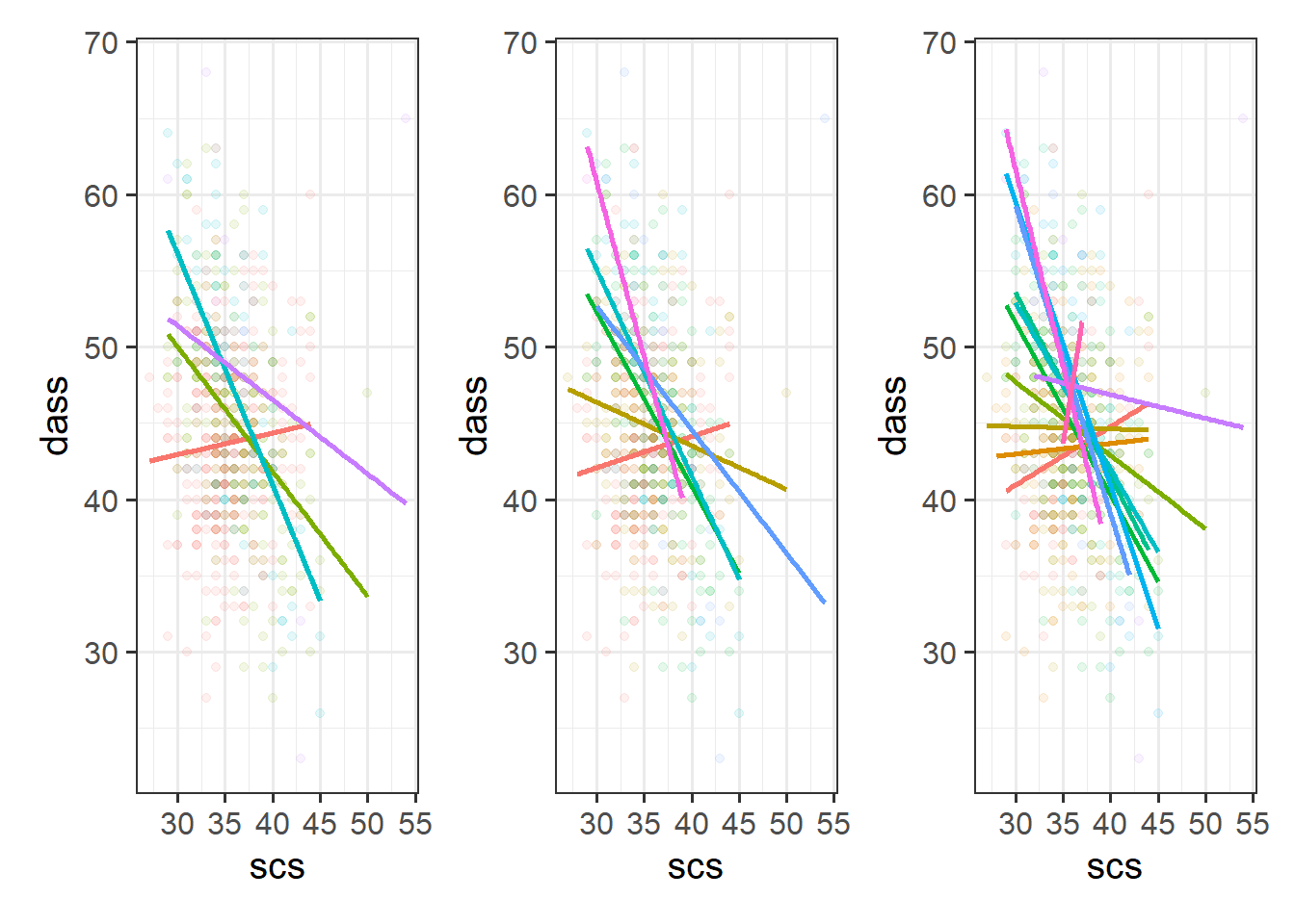
Plot the relationship between scores on the SCS and scores on the DASS-21, for each group of the variable we just created.
How does the pattern change? Does it suggest an interaction?
Tip: Rather than creating four separate plots, you might want to map some feature of the plot to the variable we created in the data, or make use of facet_wrap()/facet_grid().
Solution
ggplot(data = scs_study, aes(x = scs, y = dass, col = zn_group)) +
  geom_point() +
  facet_grid(~zn_group) +
  theme(legend.position = "none") # remove the legend
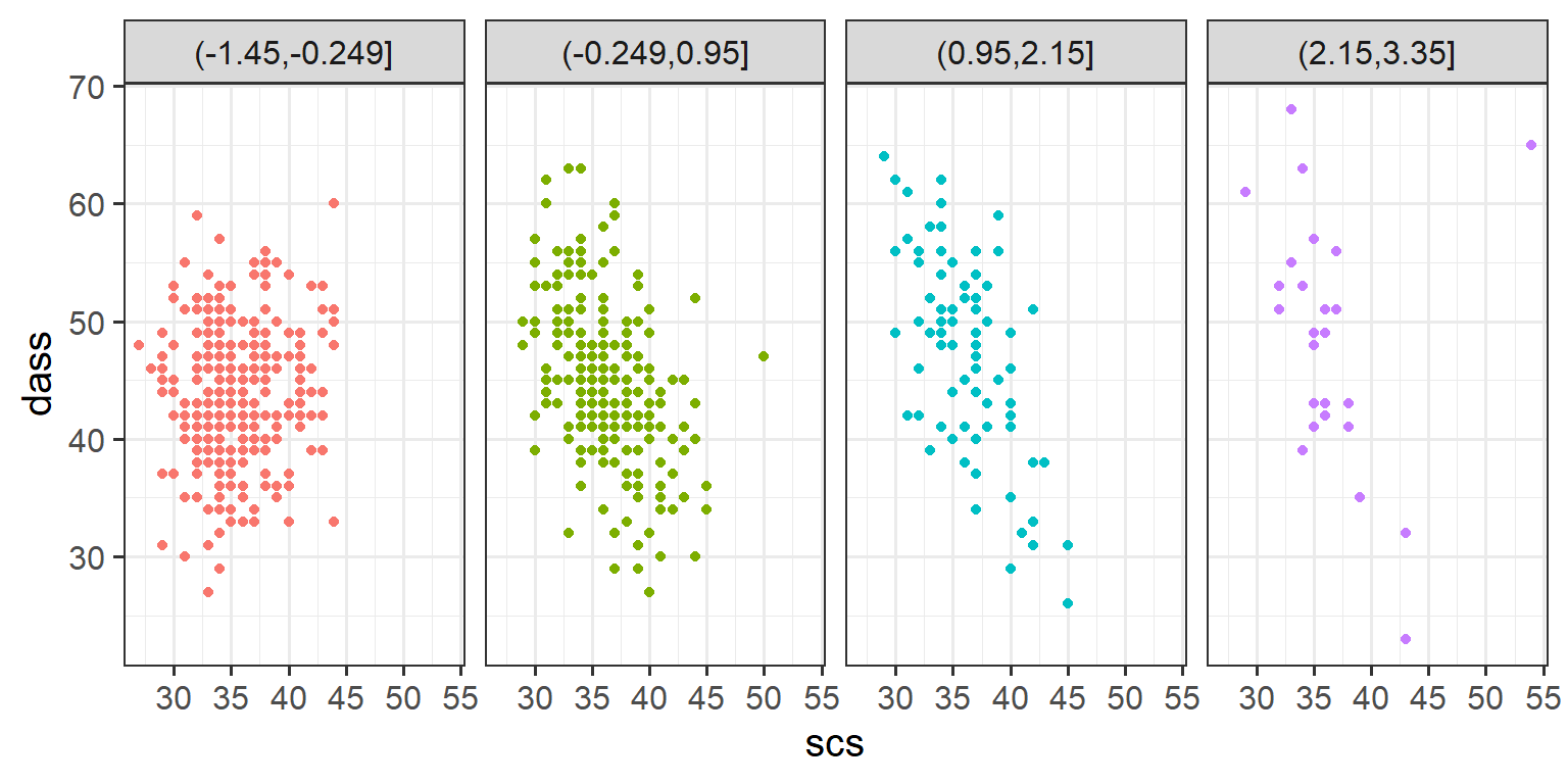
The relationship between SCS scores and DASS-21 scores appears to be different between these groups. For those with a relatively high neuroticism score, the relationship seems stronger, while for those with a low neuroticism score there is almost no discernable relationship.
This suggests an interaction - the relationship of DASS-21 ~ SCS differs across the values of neuroticism!
Cutting one of the explanatory variables up into groups essentially turns a numeric variable into a categorical one. We did this just to make it easier to visualise how a relationship changes across the values of another variable, because we can imagine a separate line for the relationship between SCS and DASS-21 scores for each of the groups of neuroticism. However, in grouping a numeric variable like this we lose information. Neuroticism is measured on a continuous scale, and we want to capture how the relationship between SCS and DASS-21 changes across that continuum (rather than cutting it into chunks).
We could imagine cutting it into more and more chunks (see Figure 1), until what we end up with is a an infinite number of lines - i.e., a three-dimensional plane/surface (recall that in for a multiple regression model with 2 explanatory variables, we can think of the model as having three-dimensions). The inclusion of the interaction term simply results in this surface no longer being necessarily flat. You can see this in Figure 2.
Question 5
Fit your model using lm().
Solution
dass_mdl <- lm(dass ~ 1 + scs*zn, data = scs_study)
summary(dass_mdl)
##
## Call:
## lm(formula = dass ~ 1 + scs * zn, data = scs_study)
##
## Residuals:
##     Min      1Q  Median      3Q     Max
## -16.301  -3.825  -0.173   3.733  45.777
##
## Coefficients:
##             Estimate Std. Error t value Pr(>|t|)
## (Intercept) 60.80887    2.45399  24.780  < 2e-16 ***
## scs         -0.44391    0.06834  -6.495 1.64e-10 ***
## zn          20.12813    2.35951   8.531  < 2e-16 ***
## scs:zn      -0.51861    0.06552  -7.915 1.06e-14 ***
## ---
## Signif. codes:  0 '***' 0.001 '**' 0.01 '*' 0.05 '.' 0.1 ' ' 1
##
## Residual standard error: 6.123 on 652 degrees of freedom
## Multiple R-squared:  0.1825, Adjusted R-squared:  0.1787
## F-statistic:  48.5 on 3 and 652 DF,  p-value: < 2.2e-16
Alternatively, as scs*zn expands to scs + zn + scs:zn, you could equivalently fit the same model as above using the following code. The two are completely equivalent and you only need to run one.
dass_mdl <- lm(dass ~ 1 + scs + zn + scs:zn, data = scs_study)
summary(dass_mdl)
Question 6
| (Intercept) |
60.8 |
2.45 |
24.8 |
5e-96 |
| scs |
-0.444 |
0.0683 |
-6.5 |
1.64e-10 |
| zn |
20.1 |
2.36 |
8.53 |
1.02e-16 |
| scs:zn |
-0.519 |
0.0655 |
-7.92 |
1.06e-14 |
Recall that the coefficients zn and scs from our model now reflect the estimated change in the outcome associated with an increase of 1 in the explanatory variables, when the other variable is zero.
Think - what is 0 in each variable? what is an increase of 1? Are these meaningful? Would you suggest recentering either variable?
Solution
The neuroticism variable zn is Z-scored, which means that 0 is the mean (it is mean-centered), and 1 is a standard deviation.
The Social Comparison Scale variable scs is the raw-score. Looking back at the description of the variables, we can work out that the minimum possible score is 11 (if people respond 1 for each of the 11 questions) and the maximum is 55 (if they respond 5 for all questions). Is it meaningful/useful to talk about estimated effects for people who score 0? Not really.
But we can make it so that zero represents something else, such as the minimum score, or the mean score. For instance, scs_study$scs - 11 will subtract 11 from the scores, making zero the minimum possible score on the scale.
Question 7
Recenter one or both of your explanatory variables to ensure that 0 is a meaningful value.
Solution
We’re going to mean-center the scores on the SCS. Think about what someone who now scores zero on the zn variable and zero on the mean-centered SCS?
scs_study <-
  scs_study %>%
  mutate(
    scs_mc = scs - mean(scs)
  )
Question 8
We re-fit the model using mean-centered SCS scores instead of the original variable. Here are the parameter estimates:
dass_mdl2 <- lm(dass ~ 1 + scs_mc * zn, data = scs_study)

# pull out the coefficients from the summary():
summary(dass_mdl2)$coefficients
##               Estimate Std. Error    t value     Pr(>|t|)
## (Intercept) 44.9324476 0.24052861 186.807079 0.000000e+00
## scs_mc      -0.4439065 0.06834135  -6.495431 1.643265e-10
## zn           1.5797687 0.24086372   6.558766 1.105118e-10
## scs_mc:zn   -0.5186142 0.06552100  -7.915236 1.063297e-14
Fill in the blanks in the statements below.
- For those of average neuroticism and who score average on the SCS, the estimated DASS-21 Score is ???
- For those who who score ??? on the SCS, an increase of ??? in neuroticism is associated with a change of 1.58 in DASS-21 Scores
- For those of average neuroticism, an increase of ??? on the SCS is associated with a change of -0.44 in DASS-21 Scores
- For every increase of ??? in neuroticism, the change in DASS-21 associated with an increase of ??? on the SCS is asjusted by ???
- For every increase of ??? in SCS, the change in DASS-21 associated with an increase of ??? in neuroticism is asjusted by ???
Solution
- For those of average neuroticism and who score average on the SCS, the estimated DASS-21 Score is 44.93
- For those who who score average (mean) on the SCS, an increase of 1 standard deviation in neuroticism is associated with a change of 1.58 in DASS-21 Scores
- For those of average neuroticism, an increase of 1 on the SCS is associated with a change of -0.44 in DASS-21 Scores
- For every increase of 1 standard deviation in neuroticism, the change in DASS-21 associated with an increase of 1 on the SCS is asjusted by -0.52
- For every increase of 1 in SCS, the change in DASS-21 associated with an increase of 1 standard deviation in neuroticism is asjusted by -0.52