Multiple linear regression basics

Information about solutions

Solutions for these exercises are available immediately below each question.
We would like to emphasise that much evidence suggests that testing enhances learning, and we strongly encourage you to make a concerted attempt at answering each question before looking at the solutions. Immediately looking at the solutions and then copying the code into your work will lead to poorer learning.
We would also like to note that there are always many different ways to achieve the same thing in R, and the solutions provided are simply one approach.

Be sure to check the solutions to last week’s exercises.
You can still ask any questions about previous weeks’ materials if things aren’t clear!

LEARNING OBJECTIVES

1. Extend the ideas of SLR to consider regression models with two or more predictors.
2. Understand and interpret the coefficients in multiple linear regression models
3. (Categorical pred.) Understand the meaning of a MLR model with categorical predictors (no interaction case). For example, two parallel regression lines, one for each of two groups.

In this block of exercises, we move from the simple linear regression model (one outcome variable, one explanatory variable) to the multiple regression model (one outcome variable, multiple explanatory variables). Everything we just learned about simple linear regression can be extended (with minor modification) to the multiple regresion model. The key conceptual difference is that for simple linear regression we think of the distribution of errors at some fixed value of the explanatory variable, and for multiple linear regression, we think about the distribution of errors at fixed set of values for all our explanatory variables.

~ Numeric + Numeric

Research question
Reseachers are interested in the relationship between psychological wellbeing and time spent outdoors.
The researchers know that other aspects of peoples’ lifestyles such as how much social interaction they have can influence their mental well-being. They would like to study whether there is a relationship between well-being and time spent outdoors after taking into account the relationship between well-being and social interactions.

Wellbeing data codebook.

Download link

The data is available at https://uoepsy.github.io/data/wellbeing.csv.

Description

Researchers interviewed 32 participants, selected at random from the population of residents of Edinburgh & Lothians. They used the Warwick-Edinburgh Mental Wellbeing Scale (WEMWBS), a self-report measure of mental health and well-being. The scale is scored by summing responses to each item, with items answered on a 1 to 5 Likert scale. The minimum scale score is 14 and the maximum is 70.
The researchers also asked participants to estimate the average number of hours they spend outdoors each week, the average number of social interactions they have each week (whether on-line or in-person), and whether they believe that they stick to a routine throughout the week (Yes/No).

The data in wellbeing.csv contain five attributes collected from a random sample of \(n=32\) hypothetical residents over Edinburgh & Lothians, and include:

• wellbeing: Warwick-Edinburgh Mental Wellbeing Scale (WEMWBS), a self-report measure of mental health and well-being. The scale is scored by summing responses to each item, with items answered on a 1 to 5 Likert scale. The minimum scale score is 14 and the maximum is 70.
  
• outdoor_time: Self report estimated number of hours per week spent outdoors
  
• social_int: Self report estimated number of social interactions per week (both online and in-person)
• routine: Binary Yes/No response to the question “Do you follow a daily routine throughout the week?”
• location: Location of primary residence (City, Suburb, Rural)

Preview

The first six rows of the data are:

wellbeing	outdoor_time	social_int	location	routine
30	7	8	Suburb	Routine
21	9	8	City	No Routine
38	14	10	Suburb	Routine
27	16	10	City	No Routine
20	1	10	Rural	No Routine
37	11	12	Suburb	No Routine

Question 1

Create a new RMarkdown, and in the first code-chunk, load the required libraries and import the wellbeing data into R. Assign them to a object called mwdata.

Solution

library(tidyverse)

# Read in data
mwdata = read_csv(file = "https://uoepsy.github.io/data/wellbeing.csv")
head(mwdata)

## # A tibble: 6 x 5
##   wellbeing outdoor_time social_int location routine   
##       <dbl>        <dbl>      <dbl> <chr>    <chr>     
## 1        30            7          8 Suburb   Routine   
## 2        21            9          8 City     No Routine
## 3        38           14         10 Suburb   Routine   
## 4        27           16         10 City     No Routine
## 5        20            1         10 Rural    No Routine
## 6        37           11         12 Suburb   No Routine

Question 2

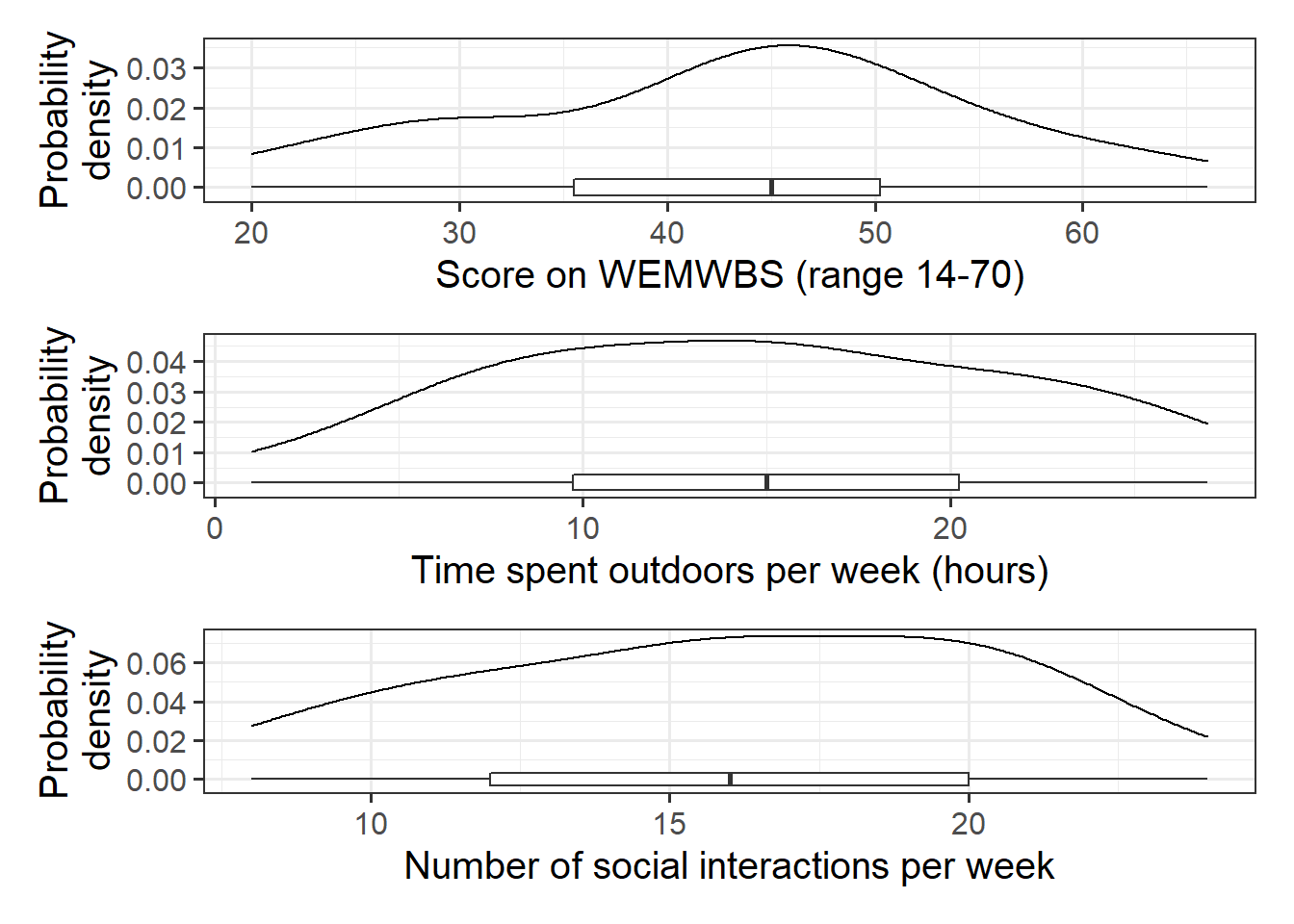
Produce plots of the marginal distributions (the distributions of each variable in the analysis without reference to the other variables) of the wellbeing, outdoor_time, and social_int variables.

Solution

We should be familiar now with how to visualise a marginal distribution. You might choose histograms, density curves, or boxplots, or a combination:

library(patchwork) #used to arrange plots

wellbeing_plot <- 
  ggplot(data = mwdata, aes(x = wellbeing)) +
  geom_density() +
  geom_boxplot(width = 1/250) +
  labs(x = "Score on WEMWBS (range 14-70)", y = "Probability\ndensity")

outdoortime_plot <- 
  ggplot(data = mwdata, aes(x = outdoor_time)) +
  geom_density() +
  geom_boxplot(width = 1/200) +
  labs(x = "Time spent outdoors per week (hours)", y = "Probability\ndensity")

social_plot <- 
  ggplot(data = mwdata, aes(x = social_int)) +
  geom_density() +
  geom_boxplot(width = 1/150) +
  labs(x = "Number of social interactions per week", y = "Probability\ndensity")

# the "patchwork" library allows us to arrange multiple plots
wellbeing_plot / outdoortime_plot / social_plot

Figure 1: Marginal distribution plots of wellbeing sores, weekly hours spent outdoors, and social interactions

• The marginal distribution of scores on the WEMWBS is unimodal with a mean of approximately 43. There is variation in WEMWBS scores (SD = 11.7).
  
• The marginal distribution of weekly hours spent outdoors is unimodal with a mean of approximately 14.8. There is variation in weekly hours spent outdoors (SD = 6.9).
  
• The marginal distribution of numbers of social interactions per week is unimodal with a mean of approximately 16. There is variation in numbers of social interactions (SD = 4.4).

Question 3

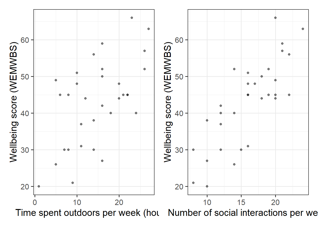
Produce plots of the marginal relationships between the outcome variable (wellbeing) and each of the explanatory variables.

Solution

wellbeing_outdoor <- 
  ggplot(data = mwdata, aes(x = outdoor_time, y = wellbeing)) +
  geom_point(alpha = 0.5) +
  labs(x = "Time spent outdoors per week (hours)", y = "Wellbeing score (WEMWBS)")

wellbeing_social <- 
  ggplot(data = mwdata, aes(x = social_int, y = wellbeing)) +
  geom_point(alpha = 0.5) +
  labs(x = "Number of social interactions per week", y = "Wellbeing score (WEMWBS)")

wellbeing_outdoor | wellbeing_social

Figure 2: Scatterplots displaying the relationships between scores on the WEMWBS and a) weekly outdoor time (hours), and b) weekly number of social interactions

Question 4

Produce a correlation matrix of the variables which are to be used in the analysis, and write a short paragraph describing the relationships.

Correlation matrix

A table showing the correlation coefficients - \(r_{(x,y)}=\frac{\mathrm{cov}(x,y)}{s_xs_y}\) - between variables. Each cell in the table shows the relationship between two variables. The diagonals show the correlation of a variable with itself (and are therefore always equal to 1).

We can create a correlation matrix easily by giving the cor() function a dataframe. However, we only want to give it 3 columns here. Think about how we select specific columns, either using select(), or giving the column numbers inside [].

Solution

We can either use:

# correlation matrix of the first 3 columns
cor(mwdata[,1:3])

or:

# select only the columns we want by name, and pass this to cor()
mwdata %>% 
  select(wellbeing, outdoor_time, social_int) %>%
  cor()

##              wellbeing outdoor_time social_int
## wellbeing    1.0000000    0.5815613  0.7939003
## outdoor_time 0.5815613    1.0000000  0.3394469
## social_int   0.7939003    0.3394469  1.0000000

There is a moderate, positive, linear relationship between weekly outdoor time and WEMWBS scores for the participants in the sample. Participants’ wellbeing scores tend to increase, on average, with the number of hours spent outdoors each week.
There is a moderate, positive, linear relationship between the weekly number of social interactions and WEMWBS scores for the participants in the sample. Participants’ wellbeing scores tend to increase, on average, with the weekly number of social interactions. There is also a weak positive correlation between weekly outdoor time and the weekly number of social interactions.

Note that there is a weak correlation between our two explanatory variables (outdoor_time and social_int). We will return to how this might affect our model when later on we look at the assumptions of multiple regression.

Question 5

The scatterplots we created above show moderate, positive, and linear relationships both between outdoor time and wellbeing, and between numbers of social interactions and wellbeing.

Specify the form of your model, where \(x_1\) = weekly outdoor time, \(x_2\) = weekly numbers of social interactions and \(y\) = scores on the WEMWBS.
What are the parameters of the model. How do we denote parameter estimates?

Solution

A model for the relationship between \(x_1\) = weekly outdoor time, \(x_2\) = weekly numbers of social interactions and \(y\) = scores on the WEMWBS is given by: \[ y = \beta_0 + \beta_1 x_1 + \beta_2 x_2 + \epsilon \\ \quad \\ \text{where} \quad \epsilon \sim N(0, \sigma) \text{ independently} \]

In the model specified above,

• \(\mu_{y|x_1, x_2} = \beta_0 + \beta_1 x + \beta_2 x_2\) represents the systematic part of the model giving the mean of \(y\) at each combination of values of \(x_1\) and \(x_2\);
• \(\epsilon\) represents the error (deviation) from that mean, and the errors are independent from one another.

The parameters of our model are:

• \(\beta_0\) (The intercept);
• \(\beta_1\) (The slope across values of \(x_1\));
• \(\beta_2\) (The slope across values of \(x_2\));
  
• \(\sigma\) (The standard deviation of the errors).

When we estimate these parameters from the available data, we have a fitted model (recall that the h\(\hat{\textrm{a}}\)ts are used to distinguish our estimates from the true unknown parameters): \[ \widehat{Wellbeing} = \hat \beta_0 + \hat \beta_1 \cdot Outdoor Time + \hat \beta_2 \cdot Social Interactions \] And we have residuals \(\hat \epsilon = y - \hat y\) which are the deviations from the observed values and our model-predicted responses.

Visual

Note that for simple linear regression we talked about our model as a line in 2 dimensions: the systematic part \(\beta_0 + \beta_1 x\) defined a line for \(\mu_y\) across the possible values of \(x\), with \(\epsilon\) as the random deviations from that line. But in multiple regression we have more than two variables making up our model.

In this particular case of three variables (one outcome + two explanatory), we can think of our model as a regression surface (See Figure 3). The systematic part of our model defines the surface across a range of possible values of both \(x_1\) and \(x_2\). Deviations from the surface are determined by the random error component, \(\hat \epsilon\).

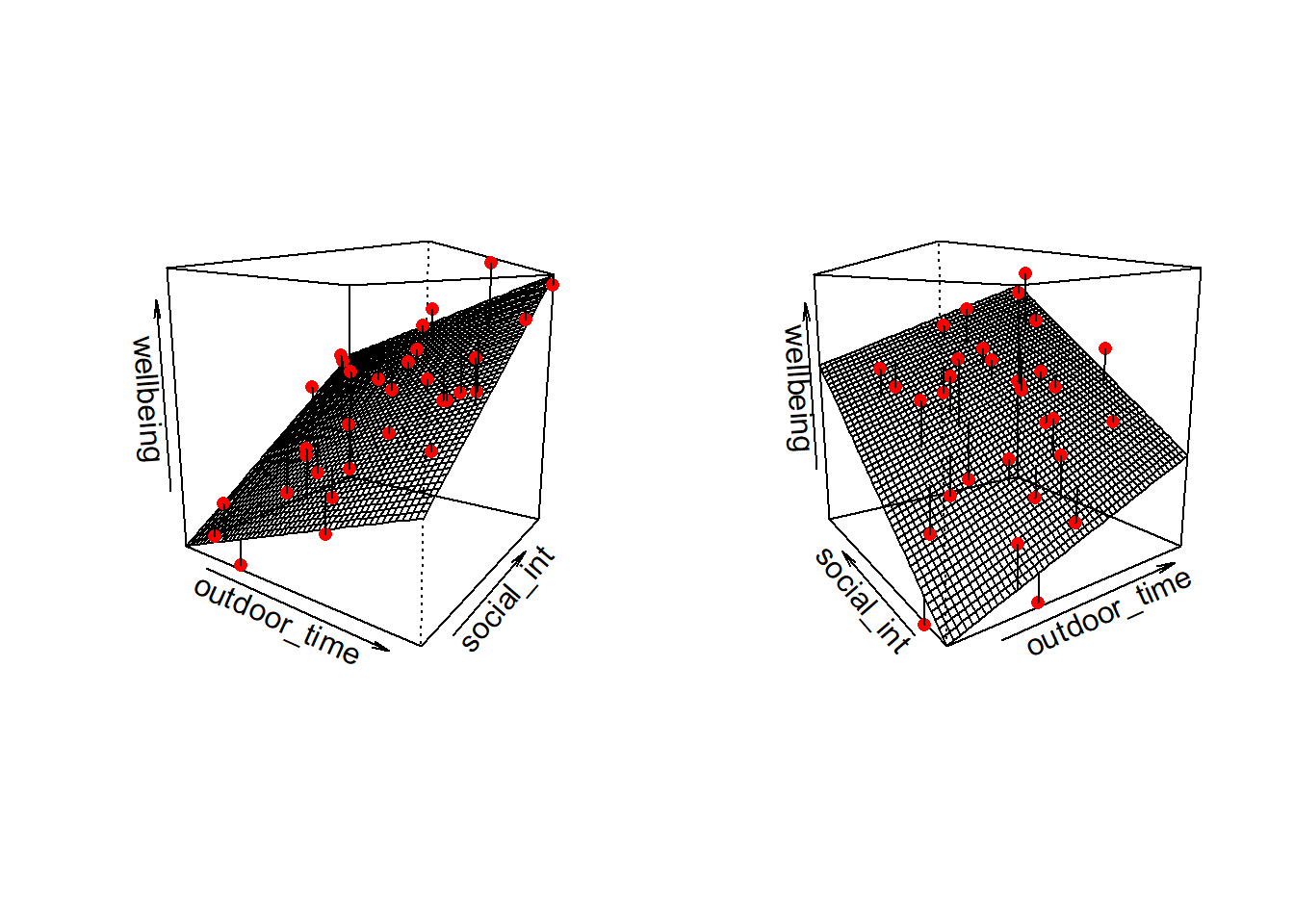
Figure 3: Regression surface for wellbeing ~ outdoor_time + social_int, from two different angles

Don’t worry about trying to figure out how to visualise it if we had any more explanatory variables! We can only concieve of 3 spatial dimensions. One could imagine this surface changing over time, which would bring in a 4th dimension, but beyond that, it’s not worth trying!.

Question 6

Fit the linear model in R, assigning the output to an object called mdl1.

As we did for simple linear regression, we can fit our multiple regression model using the lm() function. We can add as many explanatory variables as we like, separating them with a +.

lm( <response variable> ~ 1 + <explanatory variable 1> + <explanatory variable 2> + ... , data = <dataframe> )

Solution

mdl1 <- lm(wellbeing ~ 1 + outdoor_time + social_int, data = mwdata)

IMPORTANT!

You can think of the sequence of steps involved in statistical modeling as:
\[ \text{Choose} \rightarrow \text{Fit} \rightarrow \text{Assess} \rightarrow \text{Use} \]

A general rule

Do not use (draw inferences or predictions from) a model before you have assessed whether the model satisfies the underlying assumptions

So far for our multiple regression model we have completed the first two steps (Choose and Fit) in that we have:

1. Explored/visualised our data and specified our model
2. fitted the model in R.

We are going to skip straight to the Use step here, and move to interpreting our parameter estimates and construct confidence intervals around them. Please note that this when conducting real analyses, this would be an inappropriate thing to do. We will look at how to Assess whether a multiple regression model meets assumptions in a later lab.

Question 7

Using any of:

• mdl1
• mdl1$coefficients
• coef(mdl1)
• coefficients(mdl1)
• summary(mdl1)

Write out the estimated parameter values of:

1. \(\hat \beta_0\), the estimated average wellbeing score associated with zero hours of outdoor time and zero social interactions per week.
   
2. \(\hat \beta_1\), the estimated increase in average wellbeing score associated with one hour increase in weekly outdoor time, holding the number of social interactions constant (i.e., when the remaining explanatory variables are held at the same value or are fixed).
3. \(\hat \beta_2\), the estimated increase in average wellbeing score associated with an additional social interaction per week (an increase of one), holding weekly outdoor time constant.

Solution

coef(mdl1)

##  (Intercept) outdoor_time   social_int 
##    5.3703775    0.5923673    1.8034489

1. \(\hat \beta_0\) = 5.37
   
2. \(\hat \beta_1\) = 0.59
   
3. \(\hat \beta_2\) = 1.8

Interpretation of Muliple Regression Coefficients

You’ll hear a lot of different ways that people explain multiple regression coefficients.
For the model \(y = \beta_0 + \beta_1 x_1 + \beta_2 x_2 + \epsilon\), the estimate \(\hat \beta_1\) will often be reported as:

the increase in \(y\) for a one unit increase in \(x_1\) when…

• holding the effect of \(x_2\) constant.
• controlling for differences in \(x_2\).
• partialling out the effects of \(x_2\).
• holding \(x_2\) equal.
• accounting for effects of \(x_2\).

##               Estimate Std. Error  t value     Pr(>|t|)
## (Intercept)  5.3703775  4.3205141 1.242995 2.238259e-01
## outdoor_time 0.5923673  0.1689445 3.506284 1.499467e-03
## social_int   1.8034489  0.2690982 6.701825 2.369845e-07

The coefficient 0.59 of weekly outdoor time for predicting wellbeing score says that among those with the same number of social interactions per week, those who have one additional hour of outdoor time tend to, on average, score 0.59 higher on the WEMWBS wellbeing scale. The multiple regression coefficient measures that average conditional relationship.

Question 8

Within what distance from the model predicted values (the regression surface) would we expect 95% of wEMWBS wellbeing scores to be?

Hint: either sigma(mdl1) or part of the output from summary(mdl1) will help you here.

Solution

The estimated standard deviation of the errors is \(\hat \sigma\) = 6.15. We would expect 95% of wellbeing scores to be within about 12.3 (\(2 \hat \sigma\)) from the model fit.

Question 9

Obtain 95% confidence intervals for the regression coefficients, and write a sentence about each one.

Solution

confint(mdl1, level = 0.95)

##                   2.5 %     97.5 %
## (Intercept)  -3.4660660 14.2068209
## outdoor_time  0.2468371  0.9378975
## social_int    1.2530813  2.3538164

• The average wellbeing score for all those with zero hours of outdoor time and zero social interactions per week is between -3.47 and 14.21.
  
• When holding the number of social interactions per week constant, each one hour increase in weekly outdoor time is associated with a difference in wellbeing scores between 0.25 and 0.94, on average.
  
• When holding weekly outdoor time constant, each increase of one social interaction per week is associated with a difference in wellbeing scores between 1.25 and 2.35, on average.

~ Numeric + Categorical

Let’s do that again, but paying careful attention to where and how the process differs when we have a categorical (or “qualitative”) predictor.

Suppose that the group of researchers were instead wanting to study the relationship between well-being and time spent outdoors after taking into account the relationship between well-being and having a routine.

Question 10

We have already visualised the marginal distribution of weekly outdoor time in an earlier question, as well as its relationship with wellbeing scores.
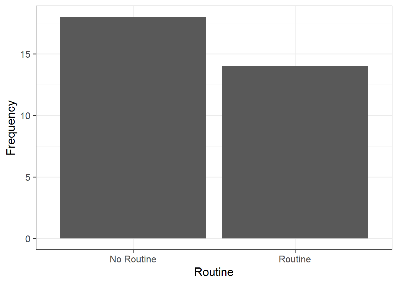
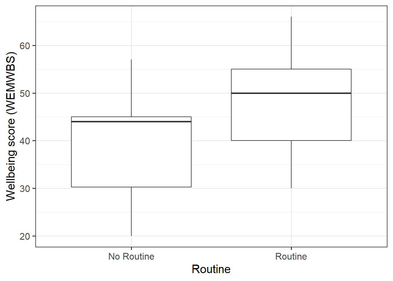
Produce visualisations of:

1. the distribution of the routine variable
2. the relationship between routine and wellbeing.

Note: We cannot visualise the distribution of routine as a density curve or boxplot, because it is a categorical variable (observations can only take one of a set of discrete response values).

Solution

geom_bar() will count the number of observations falling into each unique level of the routine variable:

ggplot(data = mwdata, aes(x = routine)) +
  geom_bar()+
  labs(x = "Routine", y = "Frequency")

Figure 4: Marginal distribution plots of Routine (y/n)

We might plot the relationship between routine and wellbeing as two boxplots:

ggplot(data = mwdata, aes(x = routine, y = wellbeing)) +
  geom_boxplot()+
  labs(x = "Routine", y = "Wellbeing score (WEMWBS)")

Figure 5: Relationship between wellbeing and presence of routine

Question 11

Fit the multiple regression model below using lm(), and assign it to an object named mdl2. Examine the summary output of the model.

\[ Wellbeing = \beta_0 + \beta_1 \cdot OutdoorTime + \beta_2 \cdot Routine + \epsilon \]

Solution

mdl2 <- lm(wellbeing ~ 1 + outdoor_time + routine, data = mwdata)
summary(mdl2)

## 
## Call:
## lm(formula = wellbeing ~ 1 + outdoor_time + routine, data = mwdata)
## 
## Residuals:
##      Min       1Q   Median       3Q      Max 
## -16.3597  -5.7983   0.1047   7.2899  12.5957 
## 
## Coefficients:
##                Estimate Std. Error t value Pr(>|t|)    
## (Intercept)     26.2525     3.9536   6.640  2.8e-07 ***
## outdoor_time     0.9152     0.2358   3.881 0.000552 ***
## routineRoutine   7.2947     3.2507   2.244 0.032633 *  
## ---
## Signif. codes:  0 '***' 0.001 '**' 0.01 '*' 0.05 '.' 0.1 ' ' 1
## 
## Residual standard error: 9.06 on 29 degrees of freedom
## Multiple R-squared:  0.4361, Adjusted R-squared:  0.3972 
## F-statistic: 11.21 on 2 and 29 DF,  p-value: 0.0002467

Question 12

\(\hat \beta_0\) (the intercept) is the estimated average wellbeing score associated with zero hours of weekly outdoor time and zero in the routine variable.

What group is the intercept the estimated wellbeing score for when they have zero hours of outdoor time? Why (think about what zero in the routine variable means)?

Solution

As you can see in the output of the model, we have a coefficient called routineRoutine. This is the parameter estimate for a dummy variable which has been inputted into the model. The lm() function will automatically name the dummy variables (and therefore the coefficients) according to what level is identified by the 1. It names them <variable><Level>, so we can tell that routineRoutine is 1 for “Routine” and 0 for “No Routine.”

The intercept is therefore the estimated wellbeing score for those with No Routine and zero hours of outdoor time.

Question 13

In the previous example, we had a visualisation of our model as a regression surface (Figure 3).
Here, one of our explanatory variables has only two possible responses. How might we visualise the model?

1. one line
2. one surface
3. two lines
4. two surfaces
5. a curved (not flat) surface

Solution

We can visualise the model \(\widehat{Wellbeing} = \hat \beta_0 + \hat \beta_1 \cdot OutdoorTime + \hat \beta_2 \cdot Routine\) as two lines.
Each line represents the model predicted values for wellbeing scores across the range of weekly outdoor time, with one line for those who report having “Routine” and one for those with “No Routine.”

Question 14

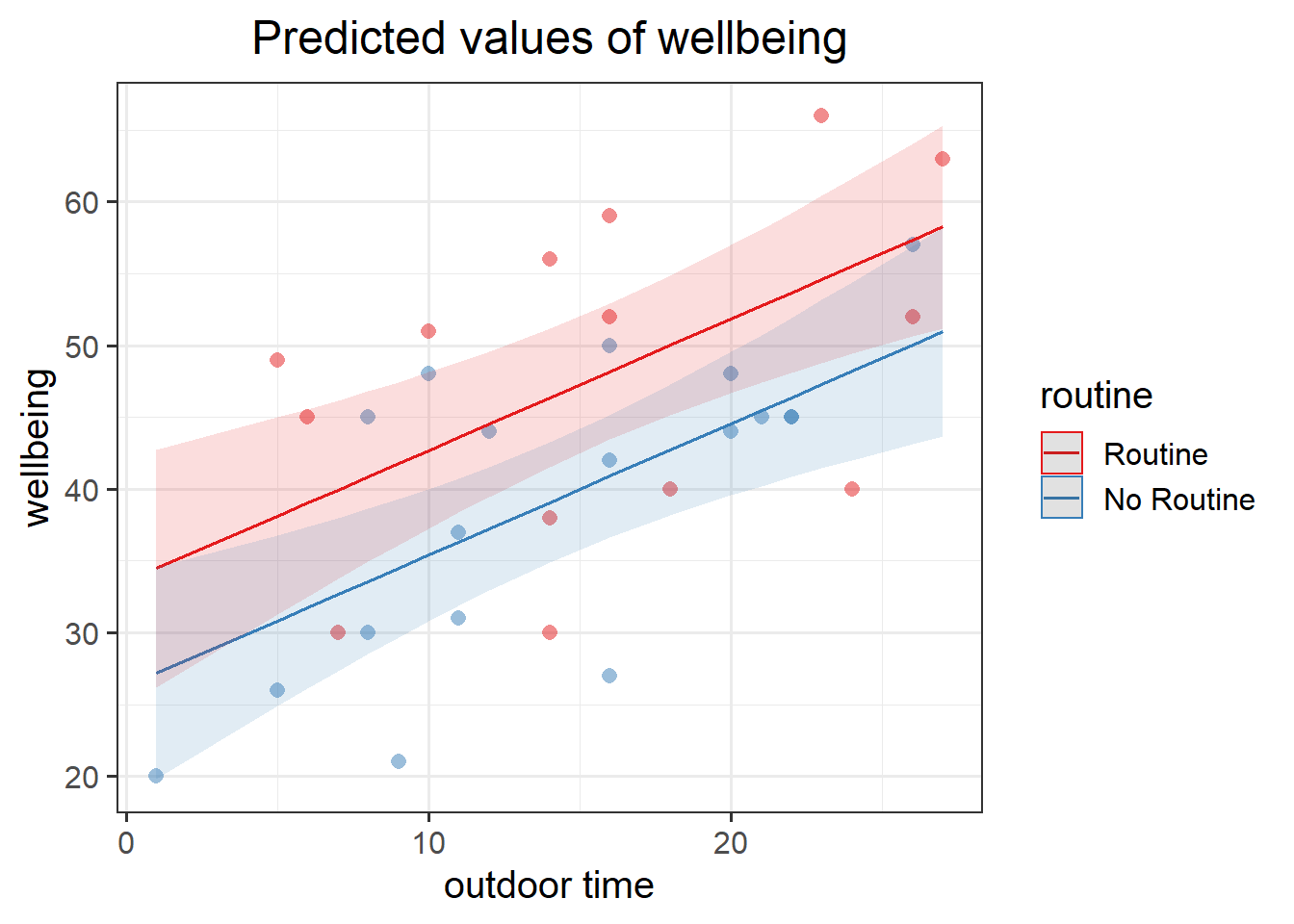
Get a pen and paper, and sketch out the plot shown in Figure 6.

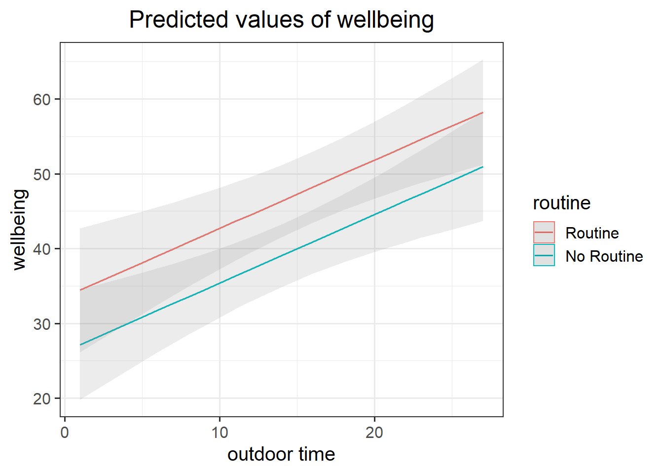
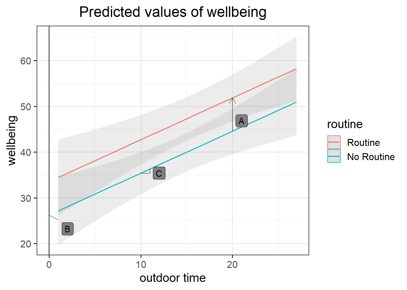
Figure 6: Multiple regression model: Wellbeing ~ Outdoor Time + Routine

Annotate your plot with labels for each of parameter estimates from your model:

Parameter Estimate	Model Coefficient	Estimate
\(\hat \beta_0\)	(Intercept)	26.25
\(\hat \beta_1\)	outdoor_time	0.92
\(\hat \beta_2\)	routineRoutine	7.29

Hint.

Below you can see where to add the labels, but we have not said which is which.

• A is the vertical distance between the red and blue lines (the lines are parallel, so this distance is the same wherever you cut it on the x-axis).
  
• B is the point at which the blue line cuts the y-axis.
  
• C is the vertical increase (increase on the y-axis) for the blue line associated with a 1 unit increase on the x-axis (the lines are parallel, so this is the same for the red line).

Solution

• A = \(\hat \beta_2\) = routineRoutine coefficient = 7.29
• B = \(\hat \beta_0\) = (Intercept) coefficient = 26.25
• C = \(\hat \beta_1\) = outdoor_time coefficient = 0.92

Question 15

Load the sjPlot package using library(sjPlot) and try running the code below. (You may already have the sjPlot package installed from previous exercises on simple linear regression, if not, you will need to install it first).

plot_model(mdl2)
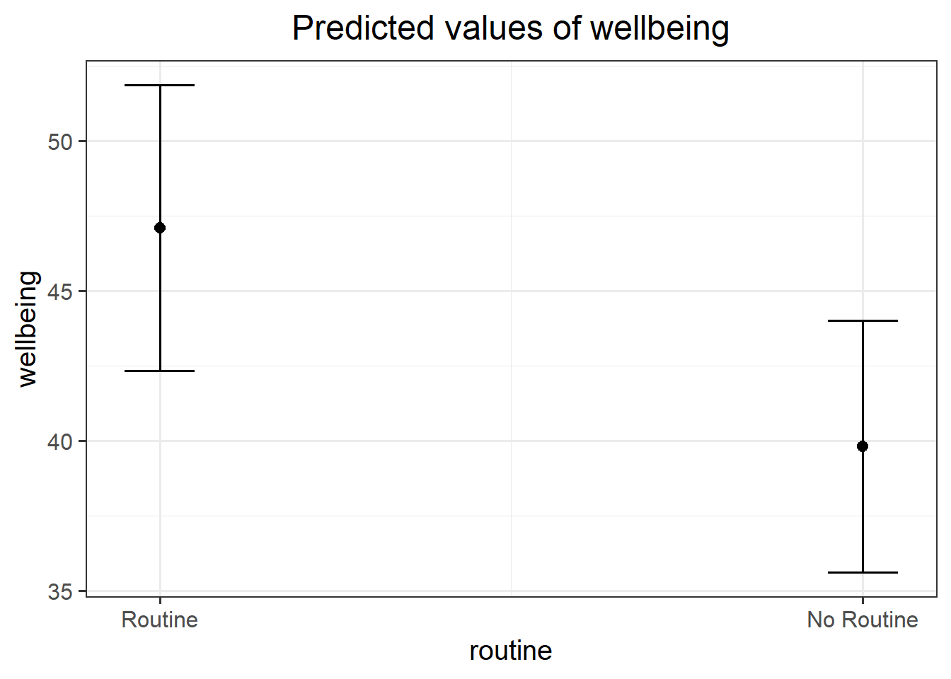
plot_model(mdl2, type = "pred")
plot_model(mdl2, type = "pred",  terms=c("outdoor_time","routine"), show.data=TRUE)

What do you think each one is showing?

The plot_model function (and the sjPlot package) can do a lot of different things. Most packages in R come with tutorials (or “vignettes”), for instance: https://strengejacke.github.io/sjPlot/articles/plot_model_estimates.html

Solution

library(sjPlot)
plot_model(mdl2)

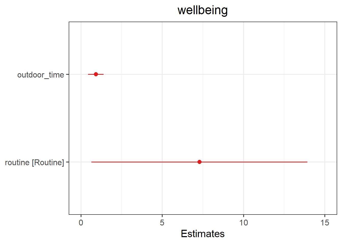These are the parameter estimates (the \(\hat \beta\)’s), and the confidence intervals.

confint(mdl2)

##                     2.5 %    97.5 %
## (Intercept)    18.1665376 34.338493
## outdoor_time    0.4329433  1.397409
## routineRoutine  0.6462090 13.943226

When we add type="pred" we are asking for the predicted values. It will provide a separate plot for each explanatory variable, showing the predicted values at each level of that variable:

plot_model(mdl2, type = "pred")

## $outdoor_time

## 
## $routine

We can combine these into one plot, and ask it to show the raw data as well:

plot_model(mdl2, type = "pred",  terms=c("outdoor_time","routine"), show.data=TRUE)

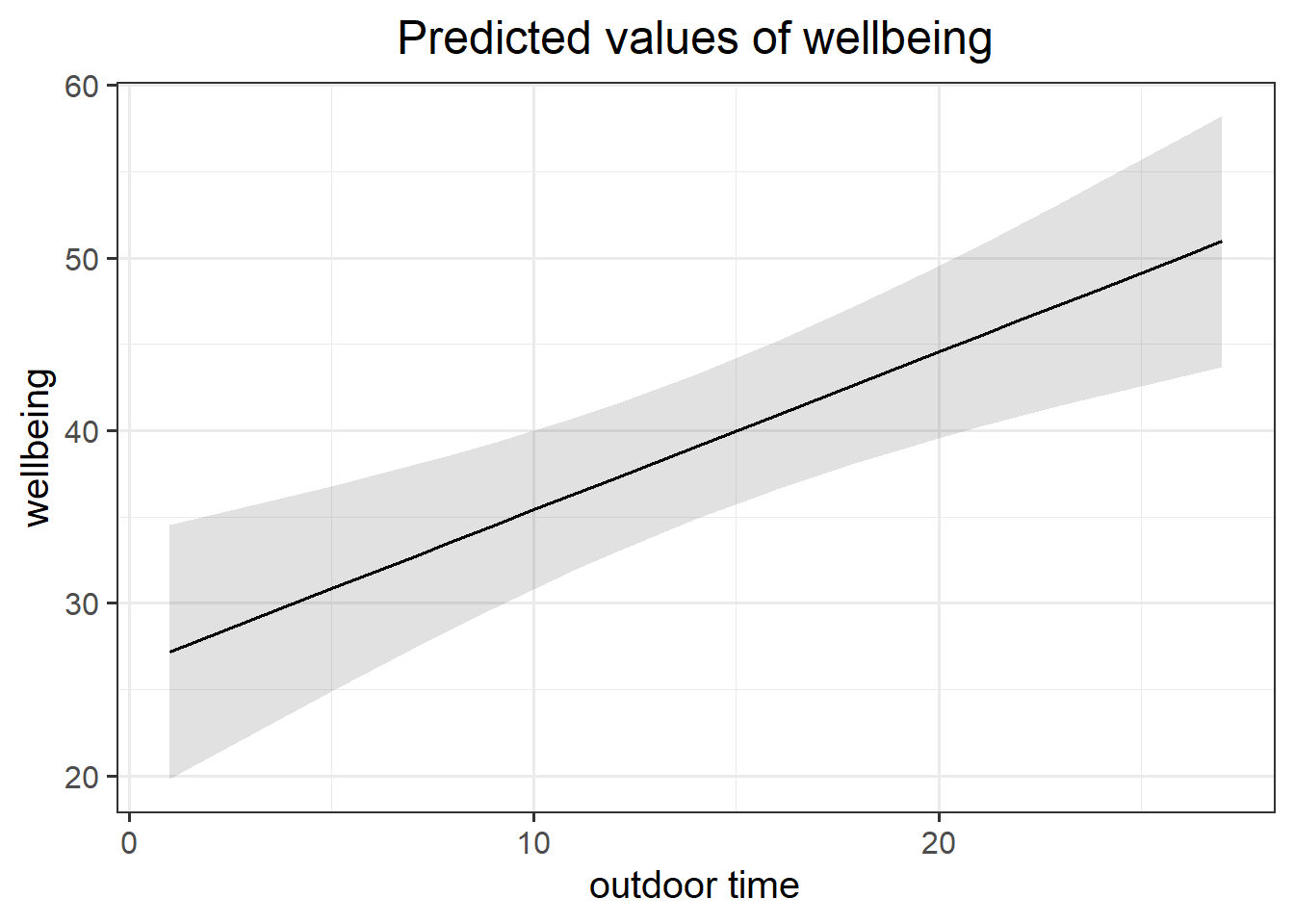
Categorical Predictors with \(k\) levels

We saw that a binary categorical variable gets inputted into our model as a variable of 0s and 1s (these typically get called “dummy variables”).

Dummy variables are numeric variables that represent categorical data.

When we have a categorical explanatory variable with more than 2 levels, our model gets a bit more - it needs not just one, but a number of dummy variables. For a categorical variable with \(k\) levels, we can express it in \(k-1\) dummy variables.

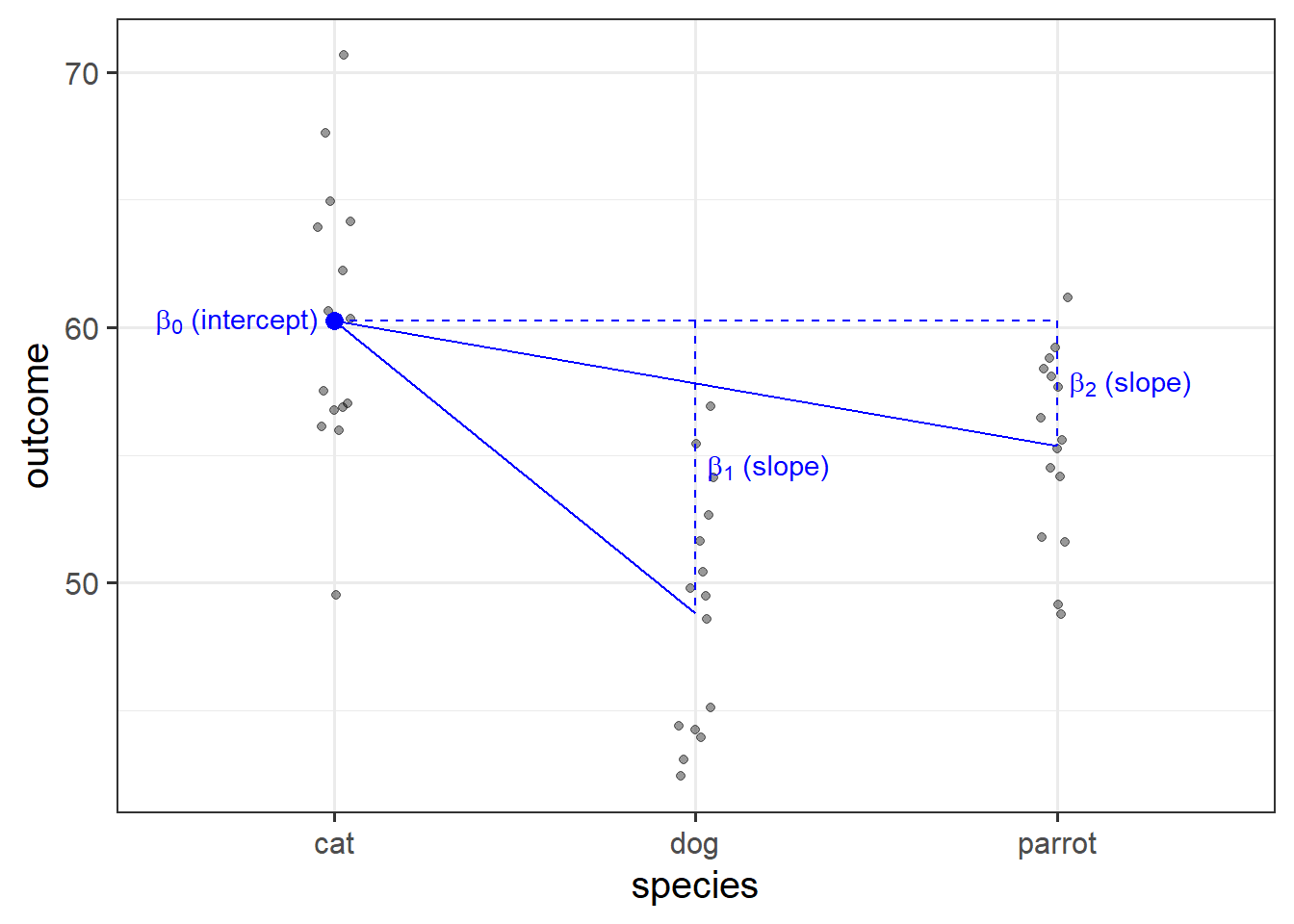
For example, the “species” column below has three levels, and can be expressed by the two variables “species_dog” and “species_parrot”:

##   species species_dog species_parrot
## 1     cat           0              0
## 2     cat           0              0
## 3     dog           1              0
## 4  parrot           0              1
## 5     dog           1              0
## 6     cat           0              0
## 7     ...         ...            ...

• The “cat” level is expressed whenever both the “species_dog” and “species_parrot” variables are 0.
• The “dog” level is expressed whenever the “species_dog” variable is 1 and the “species_parrot” variable is 0.
• The “parrot” level is expressed whenever the “species_dog” variable is 0 and the “species_parrot” variable is 1.

R will do all of this re-expression for us. If we include in our model a categorical explanatory variable with 4 different levels, the model will estimate 3 parameters - one for each dummy variable. We can interpret the parameter estimates (the coefficients we obtain using coefficients(),coef() or summary()) as the estimated increase in the outcome variable associated with an increase of one in each dummy variable (holding all other variables equal).

	Estimate	Std. Error	t value	Pr(>|t|)
(Intercept)	60.28	1.209	49.86	5.273e-39
speciesdog	-11.47	1.71	-6.708	3.806e-08
speciesparrot	-4.916	1.71	-2.875	0.006319

Note that in the above example, an increase in 1 of “species_dog” is the difference between a “cat” and a “dog.” An increase in one of “species_parrot” is the difference between a “cat” and a “parrot.” We think of the “cat” category in this example as the reference level - it is the category against which other categories are compared against.