Exploratory vs Confirmatory Data Analysis

LEARNING OBJECTIVES

1. Understand the difference between exploratory vs confirmatory analyses
2. Understand how to select models by comparing test-data MSE
3. Understand how to compute MSE via k-fold cross validation

Wine Quality

This week’s lab explores wine quality based on physiochemical properties/attributes, using data that was collected between 2004 and 2007. Specifically, the data concern white and red vinho verde.

The Data

Download the following datasets about wine quality:

• Red wine:
  https://archive.ics.uci.edu/ml/machine-learning-databases/wine-quality/winequality-red.csv
• White wine:
  https://archive.ics.uci.edu/ml/machine-learning-databases/wine-quality/winequality-white.csv

If you open them on your PC, you will notice that the data values are separated by semicolons, rather than colons. We have to tell R this by using read_delim to read a file with delimited values, and specify the delimiter by saying delim = ";":

library(tidyverse)

red <- 
    read_delim("https://archive.ics.uci.edu/ml/machine-learning-databases/wine-quality/winequality-red.csv", 
               delim = ";")

white <- 
    read_delim("https://archive.ics.uci.edu/ml/machine-learning-databases/wine-quality/winequality-white.csv", 
               delim = ";")

We will also add a column to each dataset specifying the wine color:

red <- red %>% mutate(col = "red")
white <- white %>% mutate(col = "white")

The bind_rows function is used to combine the datasets (as the name suggests, we will be combining by row). Let’s call the combined data wine:

wine <- bind_rows(
    red %>% mutate(col="red"),
    white %>% mutate(col="white")
)

Question 1

Inspect the data and check the dimensions. How many observations and how many variables are there?

Solution

# Inspect top 6 rows
head(wine)

## # A tibble: 6 x 13
##   `fixed acidity` `volatile acidity` `citric acid` `residual sugar` chlorides
##             <dbl>              <dbl>         <dbl>            <dbl>     <dbl>
## 1             7.4               0.7           0                 1.9     0.076
## 2             7.8               0.88          0                 2.6     0.098
## 3             7.8               0.76          0.04              2.3     0.092
## 4            11.2               0.28          0.56              1.9     0.075
## 5             7.4               0.7           0                 1.9     0.076
## 6             7.4               0.66          0                 1.8     0.075
## # ... with 8 more variables: free sulfur dioxide <dbl>,
## #   total sulfur dioxide <dbl>, density <dbl>, pH <dbl>, sulphates <dbl>,
## #   alcohol <dbl>, quality <dbl>, col <chr>

# Check data dimensions
dim(wine)

## [1] 6497   13

There are 6497 observations on 13 variables.

Exploratory analysis

For this section of the lab, we do not have a fixed research question and/or hypothesis, but will instead be exploring associations among variables. We have randomly selected two variables (alcohol, and col) to predict the outcome quality:

Variable	Description
quality	Quality rating of wine - assessed on a scale ranging from 0 (very bad) to 10 (excellent).
alcohol	Alcohol volume - measured as a percentage.
col	Colour of wine - red or white.

Question 2

Subset the data to only include these three variables we want to explore further - quality, alcohol, col.

Solution

wine <- wine %>%
    select(quality, alcohol, col)

Question 3

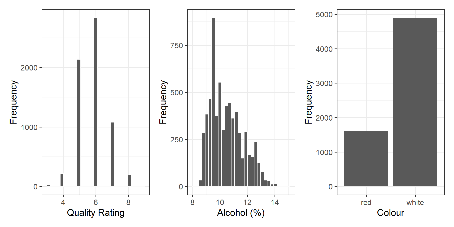
Visualise each variable individually, and note down your observations.

Solution

# To create multiple panels
library(patchwork)

# Quality Rating
p1 <- ggplot(wine, aes(x = quality)) +
    geom_histogram(color = 'white') +
    labs(x = 'Quality Rating', 
         y = 'Frequency')

# Alcohol (%)
p2 <- ggplot(wine, aes(x = alcohol)) +
    geom_histogram(color = 'white') +
    labs(x = 'Alcohol (%)', 
         y = 'Frequency')

# Colour
p3 <- ggplot(wine, aes(x = col)) + 
    geom_bar() + 
    labs(x = 'Colour', 
         y = 'Frequency')

# Stack the plots horizontally with vertical bars
p1 | p2 | p3

• Quality rating appears to be heavily set in mid-range scores (i.e., no extremely low or high)
• Alcohol (%) rather skewed, although this makes sense given that we don’t expect many wines to have a very high alcohol volume
• White wines make up the majority of the wine colours sampled - more than double that of reds

Question 4

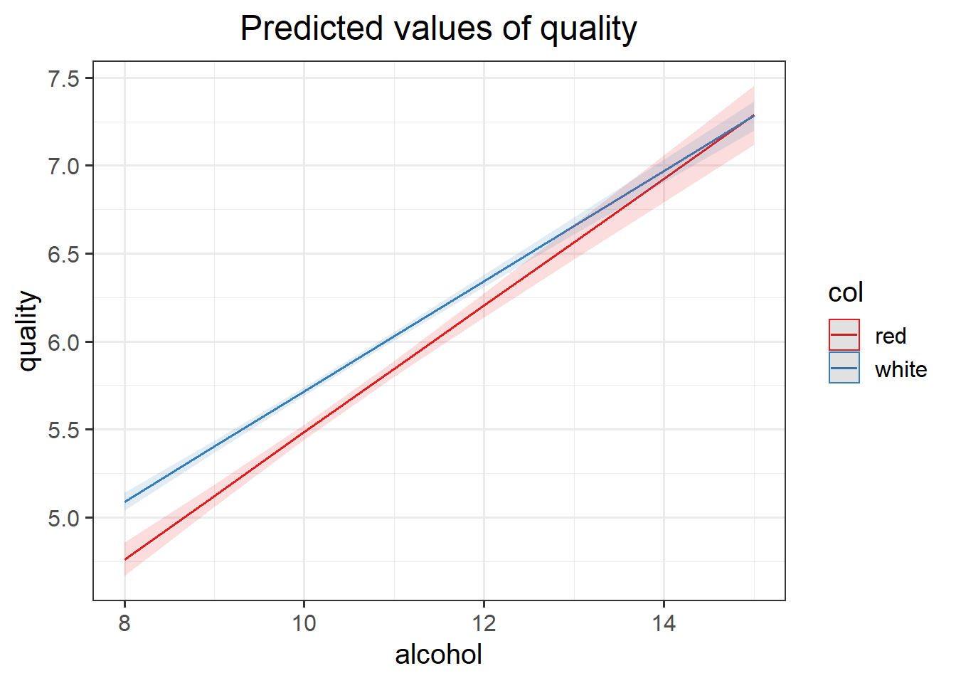
Produce a visualisation of the relationship between quality and alcohol. Consider either presenting with separate facets for wine colour, or add the colour argument within your aes() statement.

Solution

p4 <- ggplot(wine, aes(alcohol, quality)) +
    geom_point() +
    facet_wrap(~col) +
    scale_x_continuous(limits = c(5, 15)) + 
    scale_y_continuous(limits = c(0, 10)) + 
    labs(x = 'Alcohol (%)', y = 'Quality Rating')

p5 <- ggplot(wine, aes(alcohol, quality, colour = col)) +
    geom_point(size = 1, alpha = 0.5) +
    scale_x_continuous(limits = c(5, 15)) + 
    scale_y_continuous(limits = c(0, 10)) + 
    labs(x = 'Alcohol (%)', y = 'Quality Rating')

p4 | p5

From the plots, it appears that there is a positive association between alcohol percentage and quality rating. It is not so clear if there is an association between quality and colour, but white wines do seem to have more high ratings.

Our goal is to compare the following models to find if some of those variables are good predictors of quality ratings.

\[ \begin{aligned} M_A : \text{Quality} &= \beta_{A,0} + \beta_{A,1} \text{Alcohol} + \epsilon \\ M_B : \text{Quality} &= \beta_{B,0} + \beta_{B,1} \text{Col} + \epsilon \\ M_C : \text{Quality} &= \beta_{C,0} + \beta_{C,1} \text{Alcohol} + \beta_{C,2} \text{Col} + \epsilon \end{aligned} \]

To do so, we need to compute the k-fold cross validation MSE for each of those models:

\[ MSE_A = MSE(M_A) \\ MSE_B = MSE(M_B) \\ MSE_C = MSE(M_C) \]

We will begin by constructing the MSE for model A by hand, using \(k = 3\) folds.

Question 5

As a first step, we need to randomise our data, and then divide into \(k\) groups, or “folds,” of roughly equal size. We will subset into 3 groups.
Recall that we have nrow(wine), and so need to create two datasets of 2166 observations, and one with 2165 observations.

Solution

set.seed(1234)

# create the indices of the data rows and shuffle them
idx <- sample(1:nrow(wine))

# randomise the data
wine_shuffle <- wine[idx, ]

# split into three data frames 
wine1 <- wine_shuffle[1:2166, ]
wine2 <- wine_shuffle[2167:4332, ]
wine3 <- wine_shuffle[4333:6497, ]

Question 6

We are going to work through the following models:

• \(MA_{1}\): trained on bind_rows(wine2, wine3), tested on wine1
• \(MA_{2}\): trained on bind_rows(wine1, wine3), tested on wine2
• \(MA_{3}\): trained on bind_rows(wine1, wine2), tested on wine3

Recall model A involves fitting:

\[ M_A : \text{Quality} = \beta_{A,0} + \beta_{A,1} \text{Alcohol} + \epsilon \]

Solution

mA_1 <- lm(quality ~ alcohol, data = bind_rows(wine2, wine3))
mA_2 <- lm(quality ~ alcohol, data = bind_rows(wine1, wine3))
mA_3 <- lm(quality ~ alcohol, data = bind_rows(wine1, wine2))

Question 7

Calculate the test MSE on the observations in the fold that was held out. Remember that the MSE is the average squared distance between the observed and predicted values.

Solution

yhat_1 <- predict(mA_1, newdata = wine1)
yhat_2 <- predict(mA_2, newdata = wine2)
yhat_3 <- predict(mA_3, newdata = wine3)

err_1 <- wine1$quality - yhat_1
err_2 <- wine2$quality - yhat_2
err_3 <- wine3$quality - yhat_3

mseA_1 <- mean(err_1^2)
mseA_2 <- mean(err_2^2)
mseA_3 <- mean(err_3^2)

mse_A_folds <- tibble(
    Fold = 1:3,
    MSE = c(mseA_1, mseA_2, mseA_3)
)
mse_A_folds

## # A tibble: 3 x 2
##    Fold   MSE
##   <int> <dbl>
## 1     1 0.631
## 2     2 0.605
## 3     3 0.601

mse_A <- mean(mse_A_folds$MSE)
mse_A

## [1] 0.6123193

The MSE of model A is 0.61.

We now need to compute the same for the other 2 models too, in order to compare them.

For the next two models, we will use the cross-validation functions from the modelr package, as shown in the lecture.

In R, as demonstrated in the lectures, you can use the crossv_kfold() function from the modelr package to conduct K-Folding. You also need to use the map() function too.

library(modelr)

# example of three folds
CV <- crossv_kfold(wine, k = 3)
CV

## # A tibble: 3 x 3
##   train                  test                   .id  
##   <named list>           <named list>           <chr>
## 1 <resample [4,331 x 3]> <resample [2,166 x 3]> 1    
## 2 <resample [4,331 x 3]> <resample [2,166 x 3]> 2    
## 3 <resample [4,332 x 3]> <resample [2,165 x 3]> 3

Important! We selected two variables at random from the original wine dataset. If you would like more practice, feel free to ‘explore’ the associations of other variables that you think sound intriguing!

mB <- map(CV$train, ~lm(quality ~ col, data = .))
mB

## $`1`
## 
## Call:
## lm(formula = quality ~ col, data = .)
## 
## Coefficients:
## (Intercept)     colwhite  
##      5.6267       0.2642  
## 
## 
## $`2`
## 
## Call:
## lm(formula = quality ~ col, data = .)
## 
## Coefficients:
## (Intercept)     colwhite  
##      5.6645       0.2033  
## 
## 
## $`3`
## 
## Call:
## lm(formula = quality ~ col, data = .)
## 
## Coefficients:
## (Intercept)     colwhite  
##       5.617        0.258

# helper function from lecture
get_pred <- function(model, test_data){
  data = as.data.frame(test_data)
  pred = add_predictions(data, model)
  return(pred)
}

predB <- map2_df(mB, CV$test, get_pred, .id = "Run")
predB

## # A tibble: 6,497 x 5
##    Run   quality alcohol col    pred
##    <chr>   <dbl>   <dbl> <chr> <dbl>
##  1 1           5     9.8 red    5.63
##  2 1           5     9.4 red    5.63
##  3 1           5     9.1 red    5.63
##  4 1           5     9.2 red    5.63
##  5 1           5     9.3 red    5.63
##  6 1           4     9   red    5.63
##  7 1           5     9.5 red    5.63
##  8 1           5     9.4 red    5.63
##  9 1           6     9.7 red    5.63
## 10 1           5     9.4 red    5.63
## # ... with 6,487 more rows

mse_B_folds <- predB %>% 
    group_by(Run) %>%
    summarise(MSE = mean((quality - pred)^2))
mse_B_folds

## # A tibble: 3 x 2
##   Run     MSE
##   <chr> <dbl>
## 1 1     0.768
## 2 2     0.793
## 3 3     0.696

mse_B <- mean(mse_B_folds$MSE)
mse_B

## [1] 0.752463

As you see, model B leads to a MSE of 0.75.

Question 8

Calculate the MSE for model C using 3-fold cross validation.

Solution

mC <- map(CV$train, ~lm(quality ~ alcohol + col, data = .))

predC <- map2_df(mC, CV$test, get_pred, .id = "Run")
predC

## # A tibble: 6,497 x 5
##    Run   quality alcohol col    pred
##    <chr>   <dbl>   <dbl> <chr> <dbl>
##  1 1           5     9.8 red    5.43
##  2 1           5     9.4 red    5.31
##  3 1           5     9.1 red    5.21
##  4 1           5     9.2 red    5.24
##  5 1           5     9.3 red    5.27
##  6 1           4     9   red    5.18
##  7 1           5     9.5 red    5.34
##  8 1           5     9.4 red    5.31
##  9 1           6     9.7 red    5.40
## 10 1           5     9.4 red    5.31
## # ... with 6,487 more rows

mse_C_folds <- predC %>% 
    group_by(Run) %>%
    summarise(MSE = mean((quality - pred)^2))
mse_C_folds

## # A tibble: 3 x 2
##   Run     MSE
##   <chr> <dbl>
## 1 1     0.603
## 2 2     0.647
## 3 3     0.564

mse_C <- mean(mse_C_folds$MSE)
mse_C

## [1] 0.6047084

Question 9

Which model is the best model?

Solution

tibble(
    Model = c("A", "B", "C"),
    MSE = c(mse_A, mse_B, mse_C)
)

## # A tibble: 3 x 2
##   Model   MSE
##   <chr> <dbl>
## 1 A     0.612
## 2 B     0.752
## 3 C     0.605

According to the 3-fold cross validation MSE results, \(M_C\) has the lowest mean squared error: \(MSE_C =\) 0.6.

Confirmatory

You have already conducted many confirmatory analyses during the DAPR2 course - you have been asked to complete specific analyses, test pre-determined hypotheses, etc.

If you have a strong research question, and you approach the problem using an exploratory analysis approach, you may end up finding that the model with the lowest MSE is not a model that includes the variables that are required to test your hypothesis.

For example, suppose in the exploratory analysis above you also included a \(M_D\) that included the interaction between alcohol content and wine color. It could happen that the model with the lowest MSE was not \(M_D\), meaning that you would not be working with that model.

However, suppose you wanted to perform a confirmatory analysis aimed at testing whether the effect of alcohol percentage on wine quality rating is dependent on the color of the wine.

To answer such question your model must have the interaction term as the question directly relates to the interaction term.

Question 10

Fit a model that can answer the stated research hypothesis, and interpret the results.

Solution

fit <- lm(quality ~ alcohol * col, data = wine)
summary(fit)

## 
## Call:
## lm(formula = quality ~ alcohol * col, data = wine)
## 
## Residuals:
##     Min      1Q  Median      3Q     Max 
## -3.5317 -0.4973 -0.0302  0.5027  3.1579 
## 
## Coefficients:
##                  Estimate Std. Error t value Pr(>|t|)    
## (Intercept)       1.87497    0.19105   9.814  < 2e-16 ***
## alcohol           0.36084    0.01824  19.788  < 2e-16 ***
## colwhite          0.70703    0.21359   3.310 0.000937 ***
## alcohol:colwhite -0.04737    0.02034  -2.329 0.019913 *  
## ---
## Signif. codes:  0 '***' 0.001 '**' 0.01 '*' 0.05 '.' 0.1 ' ' 1
## 
## Residual standard error: 0.7768 on 6493 degrees of freedom
## Multiple R-squared:  0.209,  Adjusted R-squared:  0.2087 
## F-statistic:   572 on 3 and 6493 DF,  p-value: < 2.2e-16

library(sjPlot)
plot_model(fit, type = "int")

According to the interaction model, the effect of alcohol content on quality rating does dependent on the wine color.

The rate of change in wine quality rating seems to be significantly higher for red wines than white wines: \(t(6493) = -0.05, p = 0.02\), two-sided.