Logistic Regression II

Learning Objectives

At the end of this lab, you will:

1. Understand when to use a logistic model
2. Understand how to fit and interpret a logistic model
3. Understand how to evaluate model fit

What You Need

1. Be up to date with lectures
2. Have completed previous lab exercises from Semester 2 Week 7

Required R Packages

Remember to load all packages within a code chunk at the start of your RMarkdown file using library(). If you do not have a package and need to install, do so within the console using install.packages(" "). For further guidance on installing/updating packages, see Section C here.

For this lab, you will need to load the following package(s):

• tidyverse
• patchwork
• kableExtra
• psych
• sjPlot

Presenting Results

All results should be presented following APA guidelines.If you need a reminder on how to hide code, format tables/plots, etc., make sure to review the rmd bootcamp.

The example write-up sections included as part of the solutions are not perfect - they instead should give you a good example of what information you should include and how to structure this. Note that you must not copy any of the write-ups included below for future reports - if you do, you will be committing plagiarism, and this type of academic misconduct is taken very seriously by the University. You can find out more here.

Lab Data

You can download the data required for this lab here or read it in via this link https://uoepsy.github.io/data/QuitAttempts.csv

Study Overview

Research Question

Is attempting to quit tobacco products associated with an individuals intentions?

Smoking codebook

Description

Kalkhoran and colleagues (2015)¹ investigated predictors of dual use of cigarettes and smokeless tobacco products. Although their original sample size was large \((n = 1324)\), they were interested in running separate logistic regression analyses within subgroups. Specifically, they were interested in one of the smaller subgroups that contained subjects who used both cigarettes and smokeless tobacco products \((n=61)\).

Data Dictionary

variable	description
S	Subject Number
Q	Quit attempt - Whether the subject made an attempt to quit using tobacco products (0 = no attempt to quit; 1 = attempted to quit).
I	Individuals intention to quit (1 = Never intend to quit; 2 = May intend to quit but not in the next 6 months; 3 = Intend to quit in the next 6 months; 4 = Intend to quit in the next 30 days)

Preview

The first six rows of the data are:

S	Q	I
1	0	1
2	1	3
3	1	2
4	0	1
5	1	2
6	1	2

Setup

Setup

1. Create a new RMarkdown file
2. Load the required package(s)
3. Read in the QuitAttempts dataset into R, assigning it to an object named smoke

#load packages
library(tidyverse)
library(psych)
library(kableExtra)
library(patchwork)
library(sjPlot)

#read in data
smoke <- read_csv("https://uoepsy.github.io/data/QuitAttempts.csv")

Exercises

Study & Analysis Plan Overview

Question 1

Examine the dataset, and perform any necessary and appropriate data management steps.

Hint

• The str() function will return the overall structure of the dataset, this can be quite handy to look at
  
• Convert categorical variables to factors, and if needed, provide better variable names
• Label factors appropriately to aid with your model interpretations if required
  
• Check that the dataset is complete (i.e., are there any NA values?). We can check this using is.na()

Note that all of these steps can be done in combination - the mutate() and factor() functions will likely be useful here.

#look at structure of data:
str(smoke)

spc_tbl_ [62 × 3] (S3: spec_tbl_df/tbl_df/tbl/data.frame)
 $ S: num [1:62] 1 2 3 4 5 6 7 8 9 10 ...
 $ Q: num [1:62] 0 1 1 0 1 1 1 0 1 0 ...
 $ I: num [1:62] 1 3 2 1 2 2 3 3 3 2 ...
 - attr(*, "spec")=
  .. cols(
  ..   S = col_double(),
  ..   Q = col_double(),
  ..   I = col_double()
  .. )
 - attr(*, "problems")=<externalptr> 

#check for NAs - there are none - all FALSE:
table(is.na(smoke))

FALSE 
  186 

#re-name variables to improve clarity:
smoke <- smoke %>%
    rename(PID = S,
           Quit_Attempt = Q,
           Intention = I)

#re-assign categorical IVs as factors, and give more appropriate labels to each level:
smoke$Intention <- factor(smoke$Intention,
                              levels = c(1,2,3,4),
                              labels = c("Never", "Maybe (not in next 6 months)", "Yes (within next 6 months)", "Yes (within next 30 days)"))

Descriptive Statistics & Visualisations

Question 2

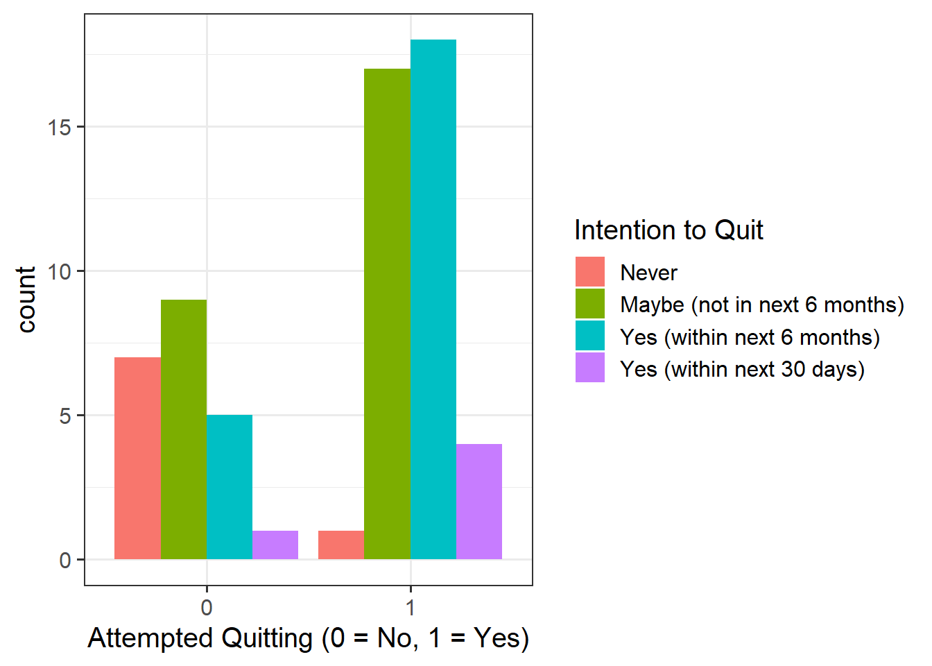
Provide a table of descriptive statistics and visualise your data.

Remember to interpret these in the context of the study.

Hint

Review the many ways to numerically and visually explore your data by reading over the data exploration flashcards.

For examples, see flashcards on descriptives statistics tables - categorical and numeric values examples.

Specifics to consider:

1. For your table of descriptive statistics, both the group_by() and summarise() functions will come in handy here

2. For your visualisations, you will need to specify as_factor() when plotting the quit attempt variable since this is numeric, but we want it to be treated as a factor only for plotting purposes

Numeric

Let’s first produce a descriptive statistics table:

smoke %>%
    select(Intention, Quit_Attempt) %>%
    table() %>%
    kable(caption = "Descriptive Statistics", col.names = c("No attempt to quit","Attempted to quit")) %>%
    kable_styling()

Table 1: Descriptive Statistics

Descriptive Statistics

	No attempt to quit	Attempted to quit
Never	7	1
Maybe (not in next 6 months)	9	17
Yes (within next 6 months)	5	18
Yes (within next 30 days)	1	4

Or alternatively we could view as proportions:

smoke_prop <- smoke %>%
  group_by(Intention, Quit_Attempt) %>%
  summarise(
    n = n()) %>%
  mutate(
    Proportion = round(n/sum(n),2)
  ) %>%
    kable(caption = "Proportions") %>%
    kable_styling()

smoke_prop 

Table 2: Proportions

Proportions

Intention	Quit_Attempt	n	Proportion
Never	0	7	0.88
Never	1	1	0.12
Maybe (not in next 6 months)	0	9	0.35
Maybe (not in next 6 months)	1	17	0.65
Yes (within next 6 months)	0	5	0.22
Yes (within next 6 months)	1	18	0.78
Yes (within next 30 days)	0	1	0.20
Yes (within next 30 days)	1	4	0.80

Based on the proportions presented in Table 2, we can see for those who had some intention to quit (i.e., maybe - not in next 6 months, yes - within next 6 months, or yes - within 30 days), there was a larger proportion of individuals who attempted to quit using tobacco products.

Visual

We can visually explore the association between the two categorical variables as follows:

smoke_plt1 <- ggplot(data = smoke, aes(x=as_factor(Quit_Attempt), fill=Intention)) +
  geom_bar(position = "dodge") +
  labs(fill = 'Intention to Quit', x = "Attempted Quitting (0 = No, 1 = Yes)")
smoke_plt1

Figure 1: Association between Intention and Quitting Attempt

From Figure 1, we can see that for those who made an attempt to quit using tobacco products, the majority intended to quit - either in the immediate or distant future. For those who made no attempt to quit using tobacco products, the majority either had no intention of quitting or did not plan to quit in the near future.

Model Fitting & Interpretation

Question 3

Fit your model using glm(), and assign it as an object with the name “smoke_mdl1”.

Hint

For an overview of how to fit a binary logistic regression model using the glm() function, see the binary logistic regression flashcard.

For an example, review the binary logistic regression - example flashcard.

smoke_mdl1 <- glm(Quit_Attempt ~ Intention, data = smoke, family = "binomial")
summary(smoke_mdl1)

Call:
glm(formula = Quit_Attempt ~ Intention, family = "binomial", 
    data = smoke)

Coefficients:
                                      Estimate Std. Error z value Pr(>|z|)   
(Intercept)                             -1.946      1.069  -1.820  0.06872 . 
IntentionMaybe (not in next 6 months)    2.582      1.146   2.253  0.02423 * 
IntentionYes (within next 6 months)      3.227      1.183   2.729  0.00636 **
IntentionYes (within next 30 days)       3.332      1.547   2.154  0.03123 * 
---
Signif. codes:  0 '***' 0.001 '**' 0.01 '*' 0.05 '.' 0.1 ' ' 1

(Dispersion parameter for binomial family taken to be 1)

    Null deviance: 80.648  on 61  degrees of freedom
Residual deviance: 68.659  on 58  degrees of freedom
AIC: 76.659

Number of Fisher Scoring iterations: 4

Question 4

Interpret your coefficients in the context of the study. When doing so, it may be useful to translate the log-odds back into odds.

Hint

For an overview of how probability, odds, and log-odds are related, review the probability, odds, and log-odds flashcard.

If you need help interpreting coefficients, review the interpretation of coefficients flashcard.

For an example, review the binary logistic regression - example flashcard.

exp(coefficients(smoke_mdl1))

                          (Intercept) IntentionMaybe (not in next 6 months) 
                            0.1428571                            13.2222222 
  IntentionYes (within next 6 months)    IntentionYes (within next 30 days) 
                           25.2000000                            28.0000000 

(Intercept)

\(\beta_0\) = (Intercept) = 0.14

• For a participant who reported that they “never intend to quit”, the odds that they did attempt quitting was 0.14.

Intention Maybe (not in next 6 months)

\(\beta_1\) = Intention Maybe (not in next 6 months) = 13.22

• Relative to those who “never intend to quit”, the odds of attempting to quit were multiplied by 13.22 for those with an “intention to quit but not in the next 6 months”.

Intention Yes (within next 6 months)

\(\beta_2\) = Intention Yes (within next 6 months) = 25.2

• Relative to those who “never intend to quit”, reporting an “intention to quit in the next 6 months” changed the odds of attempting to quit by a ratio of 25.2 .

Intention Yes (within next 30 days)

\(\beta_3\) = Intention Yes (within next 30 days) = 28

• Relative to those who “never intend to quit”, reporting an “intention to quit in the next 30 days” was associated with an increase in the odds of attempting to quit by a factor of 28.

Question 5

Calculate the predicted probability of each group attempting to quit smoking.

Hint

For an overview of how probability, odds, and log-odds are related, review the probability, odds, and log-odds flashcard.

To calculate via R, as you will see from the flashcard, you can use the predict, or plogis() functions.

For the former, you will need to specify type = "response" to obtain the predicted probabilities, and this requires the model coefficients to be in log-odds. When specifying newdata =, it might be useful to ask for each unique level of our “Intention” variable. This is very similar in procedure to how you’ve done this in the past. For a recap, see the model predicted values and residuals flashcard. For the latter, we can calculate the probability corresponding to a given value of logit(p).

Manually

The predicted probability of quitting smoking for someone who…:

• never intends to quit is = \(\frac{e^{(-1.946)}}{1 + e^{(-1.946)}}\) = 0.1250

• might intend to quit (but not in the next 6 months) is = \(\frac{e^{(-1.946+2.582)}}{1 + e^{(-1.946+2.582)}}\) = 0.6538

• intends to quit (in the next 6 months) is = \(\frac{e^{(-1.946+3.227)}}{1 + e^{(-1.946+3.227)}}\) = 0.7826

• intends to quit (in the next 30 days) is = \(\frac{e^{(-1.946+3.332)}}{1 + e^{(-1.946+3.332)}}\) = 0.8000

R Function

predict()

We can ask R to use each unique level of our “Intention” variable (which we have 4 of: “Never”, “Maybe (not in next 6 months)”, “Yes (within next 6 months)”, and “Yes (within next 30 days)”, and return the predicted probability of quitting for each:

predict(smoke_mdl1, type="response", newdata=tibble(Intention=unique(smoke$Intention)))  

        1         2         3         4 
0.1250000 0.7826087 0.6538462 0.8000000 

To check what groups the “1”, “2”, “3”, and “4” refer to, we will need to look at the ordering within unique(smoke$Intention):

unique(smoke$Intention)

[1] Never                        Yes (within next 6 months)  
[3] Maybe (not in next 6 months) Yes (within next 30 days)   
4 Levels: Never Maybe (not in next 6 months) ... Yes (within next 30 days)

So we know 1 = “Never”, 2 = “Yes (within next 6 months)”, 3 = “Maybe (not in next 6 months)”, and 4 = “Yes (within next 30 days)”.

The predicted probability of quitting smoking for someone who…:

• never intends to quit is 0.1250
• might intend to quit (but not in the next 6 months) is 0.6538
• intends to quit (in the next 6 months) is 0.7826
• intends to quit (in the next 30 days) is 0.8000

plogis()

prob_never <- plogis(-1.946)
prob_never

[1] 0.1249902

prob_maybe_not6m <- plogis(-1.946 + 2.582)
prob_maybe_not6m

[1] 0.6538487

prob_yes_6m <- plogis(-1.946 + 3.227)
prob_yes_6m

[1] 0.78262

prob_yes_30d <- plogis(-1.946 + 3.332)
prob_yes_30d

[1] 0.7999529

We can see that these values are the same (with the exception of minor rounding differences) as the predicted probabilities obtained via predict(), where the probability of attempting to quit smoking for someone who…:

• never intends to quit is 0.1250
• might intend to quit (but not in the next 6 months) is 0.6538
• intends to quit (in the next 6 months) is 0.7826
• intends to quit (in the next 30 days) is 0.8000

We can see regardless of whether we calculate manually, or via an R function, we should end up with the same predicted probabilities!

Model Fit

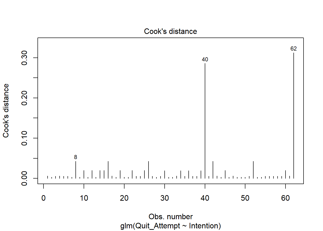
Question 6

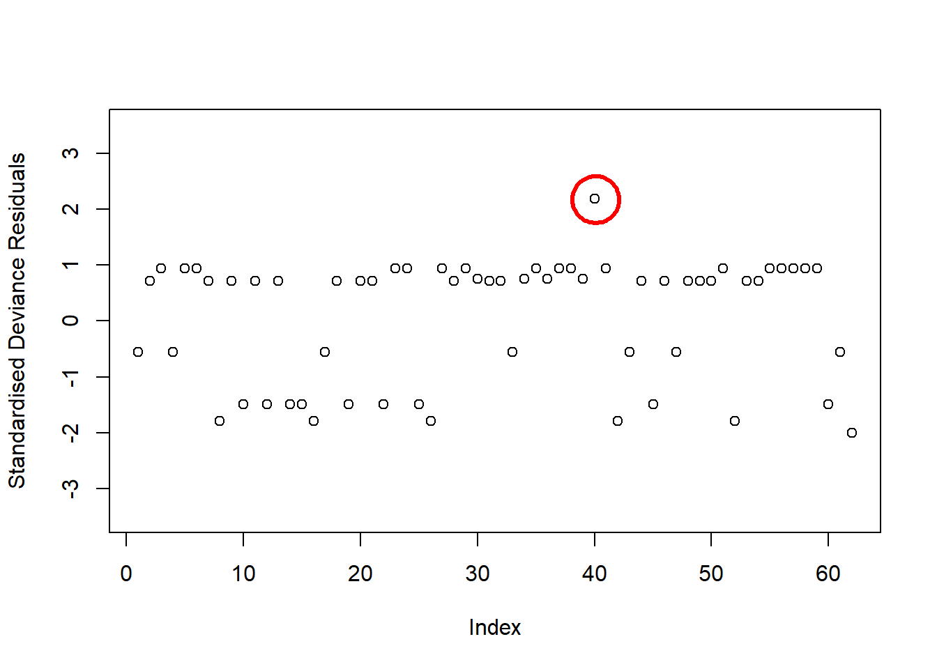
Examine the below plot to determine if the deviance residuals raise concerns about outliers:

plot(rstandard(smoke_mdl1, type = 'deviance'), ylab = 'Standardised Deviance Residuals')

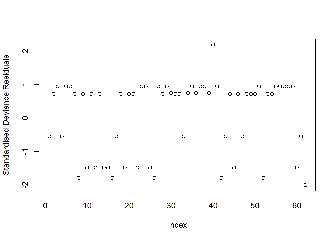
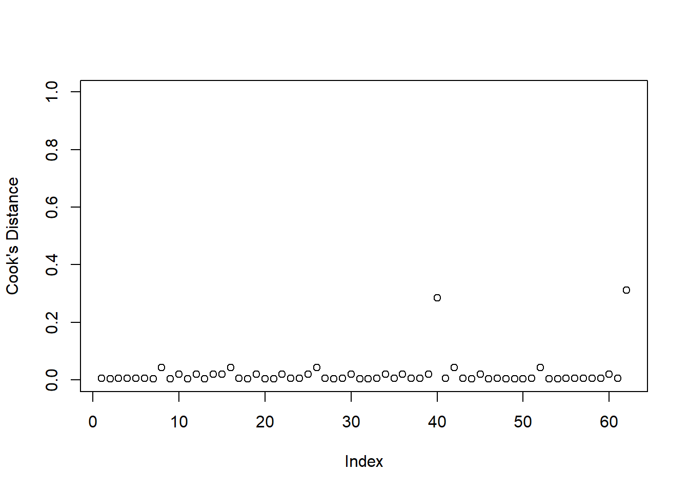
Based on this plot, are there any residuals of concern? Are there any additional plots you could check to determine if there are influential observations?

Hint

For an overview of logistic model assumptions, review the deviance residuals and high influence cases flashcards.

Deviance Residuals

In the plot of standardised deviance residuals above, there appears to be 1 residual with a value >|2|, but none with a value >|3|. We will keep this in mind and check if they are also an influential point by plotting Cook’s Distance.

Cook’s Distance

Option 1

plot(cooks.distance(smoke_mdl1), ylab = "Cook's Distance")

Option 2

plot(smoke_mdl1, which = 4)

There doesn’t appear to be any influential observations based on our Cook’s distance plot, since all values < .50.

Question 7

Perform a Deviance goodness-of-fit test to compare your fitted model to the null (denoted as \(M_1\) and \(M_0\) respectively below).

\[ \begin{aligned} \text{M}_0 &: \qquad \log \left( \frac{p}{1 - p}\right) ~=~ \beta_0 \\ \text{M}_1 &: \qquad \log \left( \frac{p}{1 - p}\right) ~=~ \beta_0 + \beta_1 \cdot \text{Intention}_\text{2} + \beta_2 \cdot \text{Intention}_\text{3} + \beta_3 \cdot \text{Intention}_\text{4} \end{aligned} \]

\[ \begin{aligned} \text{where}~{p}~ &=~ \text{probability of attempting to quit using tobacco products} \end{aligned} \]

Report the results of the model comparison in APA format, and state which model you think best fits the data.

Hint

Consider whether or not your models are nested. The model comparisons - logistic regression flashcards may be helpful to revisit.

First, let’s fit the null model:

smoke_mdl0 <- glm(Quit_Attempt ~ 1, data = smoke, family = "binomial")
summary(smoke_mdl0)

Call:
glm(formula = Quit_Attempt ~ 1, family = "binomial", data = smoke)

Coefficients:
            Estimate Std. Error z value Pr(>|z|)  
(Intercept)   0.5978     0.2654   2.252   0.0243 *
---
Signif. codes:  0 '***' 0.001 '**' 0.01 '*' 0.05 '.' 0.1 ' ' 1

(Dispersion parameter for binomial family taken to be 1)

    Null deviance: 80.648  on 61  degrees of freedom
Residual deviance: 80.648  on 61  degrees of freedom
AIC: 82.648

Number of Fisher Scoring iterations: 4

Since our models are nested, we can compare using the likelihood ratio test:

anova(smoke_mdl0, smoke_mdl1, test = 'Chisq')

Analysis of Deviance Table

Model 1: Quit_Attempt ~ 1
Model 2: Quit_Attempt ~ Intention
  Resid. Df Resid. Dev Df Deviance Pr(>Chi)   
1        61     80.648                        
2        58     68.659  3   11.989  0.00742 **
---
Signif. codes:  0 '***' 0.001 '**' 0.01 '*' 0.05 '.' 0.1 ' ' 1

At the 5% significance level, the addition of information about the participants’ intention to quit resulted in a significant decrease in model deviance \(\chi^2(3) = 11.99, p = .007\).

Hence, we have strong evidence that the model the subjects’ intention to quit is a helpful predictor of whether or not they will attempt quitting in the future.

Question 8

Check the AIC and BIC values for smoke_mdl0 and smoke_mdl1 - which model should we prefer based on these model fit indices?

Hint

Review the model comparisons - logistic regression > AIC & BIC flashcard

AIC

AIC(smoke_mdl0, smoke_mdl1)

           df      AIC
smoke_mdl0  1 82.64844
smoke_mdl1  4 76.65904

BIC

BIC(smoke_mdl0, smoke_mdl1)

           df      BIC
smoke_mdl0  1 84.77557
smoke_mdl1  4 85.16758

We used AIC and BIC model selection to distinguish between two possible models describing the association between attempting to quit and intentions. Our model with with intentions included as a predictor \((\text{AIC} = 76.66)\) was better fitting than the null model \((\text{AIC} = 82.65)\). However, the BIC values suggested that the model including intentions \((\text{BIC} = 85.17)\) was a poorer fit than the null \((\text{BIC} = 84.77)\). Based on the weight of evidence from both the Deviance goodness-of-fit test alongside the AIC and BIC values, we would conclude that the model with intentions was better fitting than the null.

Writing Up & Presenting Results

Question 9

Provide key model results in a formatted table.

Hint

Use tab_model() from the sjPlot package. For a quick guide, review the tables flashcard.

#create table for results
tab_model(smoke_mdl1,
          dv.labels = "Attempt to quit using tobacco products",
          pred.labels = c("Maybe (not in next 6 months)" = "Intend to quit but not in the next 6 months", 
                          "Yes (within next 6 months)" = "Intend to quit in the next 6 months",
                          "Yes (within next 30 days)" = "Intend to quit in the next 30 days"),
          title = "Regression table for Smoking Model")

Table 3: Regression table for Smoking Model

Regression table for Smoking Model

	Attempt to quit using tobacco products
Predictors	Odds Ratios	CI	p
(Intercept)	0.14	0.01 – 0.80	0.069
IntentionMaybe (not in next 6 months)	13.22	1.93 – 268.17	0.024
IntentionYes (within next 6 months)	25.20	3.42 – 534.12	0.006
IntentionYes (within next 30 days)	28.00	1.95 – 1181.69	0.031
Observations	62
R2 Tjur	0.192

Question 10

Interpret your results in the context of the research question and report your model in full.

Make reference to the regression table.

Hint

For an example of coefficient interpretation, review the interpretation of coefficients flashcard.

Whether or not participants made an attempt to quit using tobacco products (binary 0 vs 1; 0 no attempt to quit, 1 attempted to quit) was modeled using logistic regression, with intention to quit (‘never intend to quit’, ‘may intend to quit but not in the next 6 months’, ‘intend to quit in the next 6 months’, ‘intend to quit in the next 30 days’, with ‘never intend to quit’ as the reference level) as the only predictor. See Table 3 for full model results.

The odds of attempting to quit for the group who reported having no intention to quit were significantly less than 1 (\(Odds = 0.14,\,\, 95\%\, CI\, [0.01, 0.8]\)).

Relative to those who never intend to quit, reporting an intention to quit but not in the next 6 months was associated with 13.22 increased odds (\(95\%\, CI\, [1.93, 268.17]\)) of attempting to quit.

In comparison to those with no intention to quit, for those who intended to quit in the next six months, the odds of quitting increased were multiplied by 25.2 (\(95\%\, CI\, [3.42, 534.12]\)).

Finally, intending to quit in the next 30 days was associated with an increase in the odds of attempting to quit by a factor of 28 (\(95\%\, CI\, [1.95, 1181.69]\)) in comparison to those who never intended to quit.

In summary, having any future intention to quit was associated with increased odds of attempting to quit using tobacco products in comparison to those with no intention to quit.

Compile Report

Compile Report

Knit your report to PDF, and check over your work. To do so, you should make sure:

• Only the output you want your reader to see is visible (e.g., do you want to hide your code?)
• Check that the tinytex package is installed
• Ensure that the ‘yaml’ (bit at the very top of your document) looks something like this:

---
title: "this is my report title"
author: "B1234506"
date: "07/09/2024"
output: bookdown::pdf_document2
---

What to do if you cannot knit to PDF

If you are having issues knitting directly to PDF, try the following:

• Knit to HTML file
  
• Open your HTML in a web-browser (e.g. Chrome, Firefox)
  
• Print to PDF (Ctrl+P, then choose to save to PDF)
  
• Open file to check formatting

Hiding Code and/or Output

Hiding R Code

To not show the code of an R code chunk, and only show the output, write:

```{r, echo=FALSE}
# code goes here
```

Hiding R Output

To show the code of an R code chunk, but hide the output, write:

```{r, results='hide'}
# code goes here
```

Hiding R Code and Output

To hide both code and output of an R code chunk, write:

```{r, include=FALSE}
# code goes here
```

Tinytex

You must make sure you have tinytex installed in R so that you can “Knit” your Rmd document to a PDF file:

install.packages("tinytex")
tinytex::install_tinytex()

You should end up with a PDF file. If you have followed the above instructions and still have issues with knitting, speak with a Tutor.

Footnotes

1. Kalkhoran, S., Grana, R. A., Neilands, T. B., & Ling, P. M. (2015). Dual use of smokeless tobacco or e-cigarettes with cigarettes and cessation. American Journal of Health Behavior, 39(2), 277–284. https://doi.org/10.5993/AJHB.39.2.14