Dummy Coding

Learning Objectives

At the end of this lab, you will:

Understand how to specify a baseline/reference level for categorical variables
Understand how to specify dummy coding
Interpret the output from a model using dummy coding
Understand how to specify contrasts to test specific effects

What You Need

Be up to date with lectures

Required R Packages

Remember to load all packages within a code chunk at the start of your RMarkdown file using library(). If you do not have a package and need to install, do so within the console using install.packages(" "). For further guidance on installing/updating packages, see Section C here.

For this lab, you will need to load the following package(s):

tidyverse
psych
kableExtra
emmeans

Presenting Results

All results should be presented following APA guidelines.If you need a reminder on how to hide code, format tables/plots, etc., make sure to review the rmd bootcamp.

The example write-up sections included as part of the solutions are not perfect - they instead should give you a good example of what information you should include and how to structure this. Note that you must not copy any of the write-ups included below for future reports - if you do, you will be committing plagiarism, and this type of academic misconduct is taken very seriously by the University. You can find out more here.

Lab Data

You can download the data required for this lab here or read it in via this link https://uoepsy.github.io/data/caffeinedrink.csv

Study Overview

Research Question

Does WPM differ by caffeine treatment condition?

To investigate if the number of words typed per minute (WPM) differs among caffeine treatment conditions, the researchers conducted an experiment where participants were randomly allocated to one of four treatment conditions. Two of these conditions included non-caffeinated drinks - control (water) and mint tea, and the other two caffeinated drinks - coffee and red bull.

Drink	Caffeine	Temp
Control (Water)	No	Cold
Red Bull	Yes	Cold
Coffee	Yes	Hot
Mint Tea	No	Hot

In addition to the above research question, the researchers were also interested in the following:

Comparisons

Whether having some kind of caffeine (i.e., red bull or coffee), rather than no caffeine (i.e., control - water or mint tea), resulted in a difference in average WPM

Whether there was a difference in average WPM between those with hot drinks (i.e., mint tea / coffee) in comparison to those with cold drinks (control - water / red bull)

Caffeine data codebook

variable	description
treatment	which one of four treatment conditions the participant was assigned - control (water), coffee, mint_tea, or red_bull
wpm	average number of words typed per minute

treatment	wpm
control	109.43
control	113.83
control	113.22
control	110.46
control	116.23
control	113.12

Setup

Create a new RMarkdown file
Load the required package(s)
Read the caffeinedrink dataset into R, assigning it to an object named caffeine

Exercises

Study & Analysis Plan Overview

Question 1

Examine the dataset, and perform any necessary and appropriate data management steps.

Hint

The str() function will return the overall structure of the dataset, this can be quite handy to look at
Convert categorical variables to factors, and if needed, provide better variable names*
Label factors appropriately to aid with your model interpretations if required*
Check that the dataset is complete (i.e., are there any NA values?). We can check this using is.na()
Are scores within possible ranges (e.g., if we recorded people’s age, it would be impossible to have someone aged -31!)

*See the Overview (numeric outcomes & categorical predictors) flashcard.

Question 2

Choose an appropriate reference level for the Treatment condition.

Question 3

Provide a brief overview of the study design and data, before detailing your analysis plan to address the research question.

Hint

Give the reader some background on the context of the study
State what type of analysis you will conduct in order to address the research question
Specify the model to be fitted to address the research question (note that you will need to specify the reference level of your categorical variable)
Specify your chosen significance ($\alpha$) level
State your hypotheses

Much of the information required can be found in the Study Overview codebook. The statistical models flashcards may also be useful to refer to.

Descriptive Statistics & Visualisations

Question 4

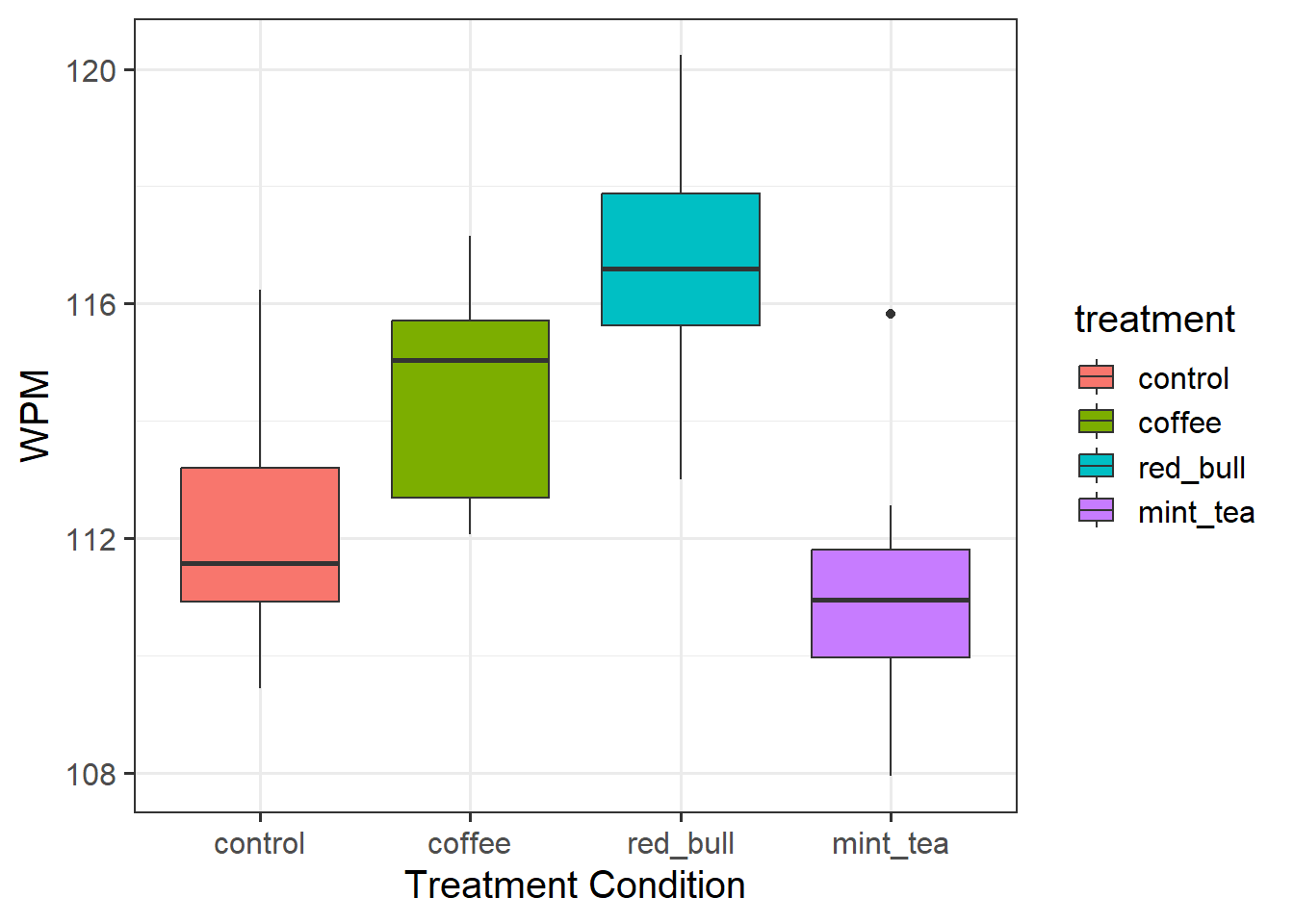
Provide a table of descriptive statistics and visualise your data.

Remember to interpret your plot in the context of the study (i.e., comment on any observed differences among treatment groups).

Hint

Review the many ways to numerically and visually explore your data by reading over the data exploration flashcards.

For examples, see flashcards on descriptives statistics tables - categorical and numeric values examples and data visualisation - bivariate examples, paying particular attention to the type of data that you’re working with.

Make sure to comment on any observed differences among the sample means of the four treatment conditions.

Descriptive Statistics
treatment	n	Mean	SD	Minimum	Maximum
control	10	112.15	1.98	109.43	116.23
coffee	10	114.48	1.82	112.07	117.16
red_bull	10	116.65	2.15	113.00	120.24
mint_tea	10	111.09	2.13	107.94	115.82

Model Fitting & Interpretation

Question 5

Fit the specified model, and assign it the name “caf_mdl1”.

Interpret your coefficients in the context of the study.

Hint

We can fit our multiple regression model using the lm() function. For a recap, see the statistical models flashcards.

Recall that R computes the dummy variables for us. Thus, each row in the summary() output of the model will correspond to one of the estimated $\beta$’s in the equation above. For a more in-depth recap, see the numeric outcomes & categorical predictors flashcards

#fit model
caf_mdl1 <- lm(wpm ~ treatment, data=caffeine)

#check model output
summary(caf_mdl1)


Call:
lm(formula = wpm ~ treatment, data = caffeine)

Residuals:
   Min     1Q Median     3Q    Max 
-3.652 -1.362 -0.151  1.125  4.729 

Coefficients:
                  Estimate Std. Error t value Pr(>|t|)    
(Intercept)       112.1460     0.6402 175.179  < 2e-16 ***
treatmentcoffee     2.3350     0.9053   2.579   0.0141 *  
treatmentred_bull   4.5060     0.9053   4.977 1.61e-05 ***
treatmentmint_tea  -1.0550     0.9053  -1.165   0.2516    
---
Signif. codes:  0 '***' 0.001 '**' 0.01 '*' 0.05 '.' 0.1 ' ' 1

Residual standard error: 2.024 on 36 degrees of freedom
Multiple R-squared:  0.5563,    Adjusted R-squared:  0.5194 
F-statistic: 15.05 on 3 and 36 DF,  p-value: 1.651e-06

Let’s first map our coefficients and estimates:

Coefficient	Estimate	Relation between $\beta$ and $\mu$
(Intercept)	112.1460	$\beta_0 = \hat \mu_1$
treatmentcoffee	2.3350	$\beta_0 + \beta_1 = \hat \mu_2$
treatmentred_bull	4.5060	$\beta_0 + \beta_2 = \hat \mu_3$
treatmentmint_tea	-1.0550	$\beta_0 + \beta_3 = \hat \mu_4$

The estimate corresponding to (Intercept) contains $\hat \beta_0 = \hat \mu_1 = 112.15$. The estimated average WPM for those in the control condition (water) was approximately 112.15.
The next estimate corresponds to treatmentcoffee and was $\hat \beta_1 = 2.34$. The difference in mean WPM between Control and Coffee was estimated to be $2.34$. Thus, $\hat \mu_2 = 112.15 + 2.34 = 114.49$. In other words, people who have had coffee typed approximately 114.49 words, which was 2.34 words per minute more than those who have had water. This difference was statistically significant $(p = .01)$.
The estimate corresponding to treatmentred_bull was $\hat \beta_2 = 4.51$. This was the estimated difference in mean WPM between Control and Red Bull, estimated to be $4.51$. Thus, $\hat \mu_3 = 112.15 + 4.51 = 116.66$. In other words, people who had red bull typed approximately 116.66 words, 4.51 words per minute more than those who had water. This difference was statistically significant $(p < .001)$.
The estimate corresponding to treatmentmint_tea was $\hat \beta_3 = -1.06$. This was the estimated difference in mean WPM between Control and Mint Tea, estimated to be $-1.06$. Thus, $\hat \mu_4 = 112.15 + (-1.06) = 111.09$. In other words, people who had mint tea typed approximately 111.09 words, 1.06 words per minute less than those who had water. This difference was not statistically significant $(p = .25)$.

Planned Comparisons / Contrasts

Question 6

Formally state the two planned comparisons that the researchers were interested in as testable hypotheses.

Hint

See the manual contrasts flashcards.

Question 7

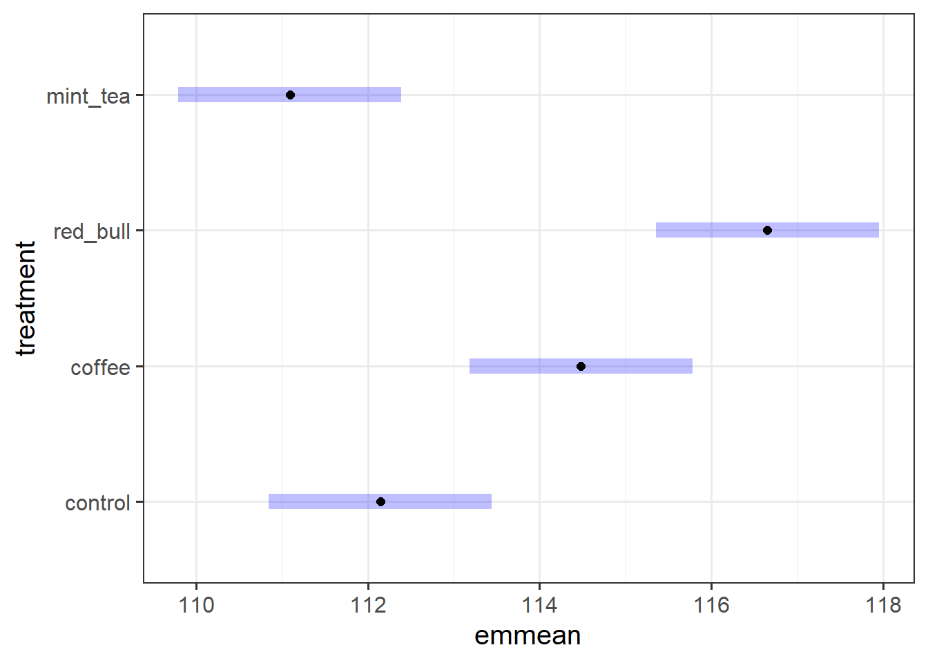
After checking the levels of the factor treatment, use emmeans() to obtain the estimated treatment means and uncertainties for your factor.

Hint

See the manual contrasts flashcards.

Question 8

Specify the coefficients of the comparisons and run the contrast analysis, obtaining 95% confidence intervals.

Hint

See the manual contrasts flashcards.

Remember that ordering matters here - look again at the output of levels(caffeine$treatment) as this will help you when assigning your weights.

Question 9

Interpret the results of the contrast analysis in the context of the researchers hypotheses.

Hint

See the manual contrasts flashcards.

Study Design

Question 10

For each of the below experiment descriptions, note (1) the design, (2) number of variables of interest, (3) levels of categorical variables, (4) what you think the reference group should be and why.

A group of researchers were interested in whether sleep deprivation influenced reaction time. They hypothesised that sleep deprived individuals would have slower reaction times than non-sleep deprived individuals.

To test this, they recruited 60 participants who were matched on a number of demographic variables including age and sex. One member of each pair (e.g., female, aged 18) was placed into a different sleep condition - ‘Sleep Deprived’ (4 hours per night) or ‘Non-Sleep Deprived’ (8 hours per night).

A group of researchers were interested in replicating an experiment testing the Stroop Effect.

They recruited 50 participants who took part in Task A (word colour and meaning are congruent) and Task B (word colour and meaning are incongruent) where they were asked to name the color of the ink instead of reading the word. The order of presentation was counterbalanced across participants. The researchers hypothesised that participants would take significantly more time (‘response time’ measured in seconds) to complete Task B than Task A.

You can test yourself here for fun: Stroop Task

A group of researchers wanted to test a hypothesised theory according to which patients with amnesia will have a deficit in explicit memory but not implicit memory. Huntingtons patients, on the other hand, will display the opposite: they will have no deficit in explicit memory, but will have a deficit in implicit memory.

To test this, researchers designed a study that included two variables: ‘Diagnosis’ (Amnesic, Huntingtons, Control) and ‘Task’ (Grammar, Classification, Recognition) where participants were randomly assigned to a Task condition. The first two tasks (Grammar and Classification) are known to reflect implicit memory processes, whereas the Recognition task is known to reflect explicit memory processes.

Compile Report

Knit your report to PDF, and check over your work. To do so, you should make sure:

Only the output you want your reader to see is visible (e.g., do you want to hide your code?)
Check that the tinytex package is installed
Ensure that the ‘yaml’ (bit at the very top of your document) looks something like this:

---
title: "this is my report title"
author: "B1234506"
date: "07/09/2024"
output: bookdown::pdf_document2
---

What to do if you cannot knit to PDF

If you are having issues knitting directly to PDF, try the following:

Knit to HTML file
Open your HTML in a web-browser (e.g. Chrome, Firefox)
Print to PDF (Ctrl+P, then choose to save to PDF)
Open file to check formatting

Hiding Code and/or Output

To not show the code of an R code chunk, and only show the output, write:

```{r, echo=FALSE}
# code goes here
```

To show the code of an R code chunk, but hide the output, write:

```{r, results='hide'}
# code goes here
```

To hide both code and output of an R code chunk, write:

```{r, include=FALSE}
# code goes here
```

Tinytex

You must make sure you have tinytex installed in R so that you can “Knit” your Rmd document to a PDF file:

install.packages("tinytex")
tinytex::install_tinytex()