| variable | description |
|---|---|
| age | Age in years of respondent |
| outdoor_time | Self report estimated number of hours per week spent outdoors |
| social_int | Self report estimated number of social interactions per week (both online and in-person) |
| routine | Binary 1=Yes/0=No response to the question 'Do you follow a daily routine throughout the week?' |
| wellbeing | Warwick-Edinburgh Mental Wellbeing Scale (WEMWBS), a self-report measure of mental health and well-being. The scale is scored by summing responses to each item, with items answered on a 1 to 5 Likert scale. The minimum scale score is 14 and the maximum is 70 |
| location | Location of primary residence (City, Suburb, Rural) |
| steps_k | Average weekly number of steps in thousands (as given by activity tracker if available) |
Assumptions and Diagnostics
Learning Objectives
At the end of this lab, you will:
- Be able to state the assumptions underlying a linear model
- Specify the assumptions underlying a linear model with multiple predictors
- Assess if a fitted model satisfies the assumptions of your model
- Assess the effect of influential cases on linear model coefficients and overall model evaluations
What You Need
- Be up to date with lectures
- Have completed Week 2 lab exercises
Required R Packages
Remember to load all packages within a code chunk at the start of your RMarkdown file using library(). If you do not have a package and need to install, do so within the console using install.packages(" "). For further guidance on installing/updating packages, see Section C here.
For this lab, you will need to load the following package(s):
- tidyverse
- car
- performance
- kableExtra
- sjPlot
Presenting Results
All results should be presented following APA guidelines.If you need a reminder on how to hide code, format tables/plots, etc., make sure to review the rmd bootcamp.
The example write-up sections included as part of the solutions are not perfect - they instead should give you a good example of what information you should include and how to structure this. Note that you must not copy any of the write-ups included below for future reports - if you do, you will be committing plagiarism, and this type of academic misconduct is taken very seriously by the University. You can find out more here.
Lab Data
You can download the data required for this lab here or read it in via this link https://uoepsy.github.io/data/wellbeing_rural.csv
Lab Overview
In the previous labs, we have fitted a number of regression models, including some with multiple predictors. In each case, we first specified the model, then visually explored the marginal distributions and associations among variables which would be used in the analysis. Finally, we fit the model, and began to examine the fit by studying what the various parameter estimates represented, and the spread of the residuals.
But before we draw inferences using our model estimates or use our model to make predictions, we need to be satisfied that our model meets a specific set of assumptions. If these assumptions are not satisfied, the results will not hold.
In this lab, we will check the assumptions of one of the multiple linear regression models that we have previously fitted in Block 1 using the ‘mwdata’ dataset (see Week 2).
Study Overview
Research Question
Is there an association between wellbeing and time spent outdoors after taking into account the association between wellbeing and social interactions?
Setup
Setup
- Create a new RMarkdown file
- Load the required package(s)
- Read the wellbeing dataset into R, assigning it to an object named
mwdata - Fit the following model:
\[ \text{Wellbeing} = \beta_0 + \beta_1 \cdot \text{Social Interactions} + \beta_2 \cdot \text{Outdoor Time} + \epsilon \]
Exercises
Assumptions
Question 1
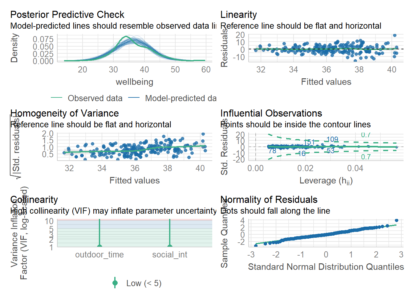
Let’s start by using check_model() for our wb_mdl1 model - we can refer to these plots as a guide as we work through the assumptions questions of the lab.
Hint
These plots cannot be used in your reports - they are to be used as a guide only.
Question 2
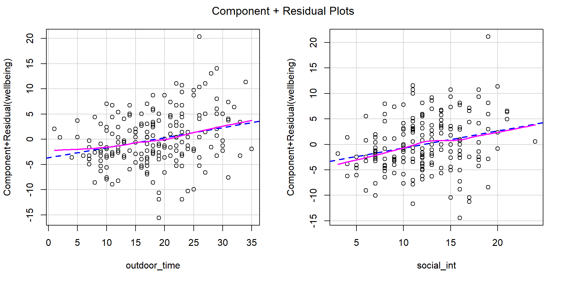
Check if the fitted model satisfies the linearity assumption for wb_mdl1.
Write a sentence summarising whether or not you consider the assumption to have been met. Justify your answer with reference to the plots.
Hint
How you check this assumption depends on the number of predictors in your model:
- Single predictor: Use either residual vs fitted values plot (
plot(model, which = 1)), and/or a scatterplot with loess lines
- Multiple predictors: Use component-residual plots (also known as partial-residual plots) to check the assumption of linearity
For more information, as well as tips to aid your interpretation, review the linearity flashcard.
Question 3
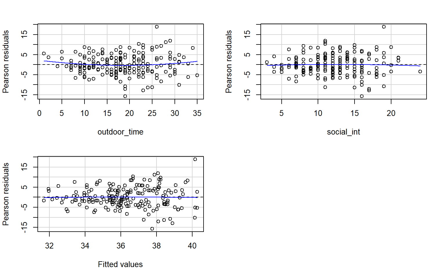
Check if the fitted model wb_mdl1 satisfy the equal variance (homoscedasticity) assumption.
Write a sentence summarising whether or not you consider the assumption to have been met. Justify your answer with reference to the plot.
Hint
Use residualPlots() to plot residuals against the predictor. Since we are only interested in visually assessing our assumption checks, we can suppress the curvature test output by specifying tests = FALSE.
For more information, as well as tips to aid your interpretation, review the equal variances (homoscedasticity) flashcard.
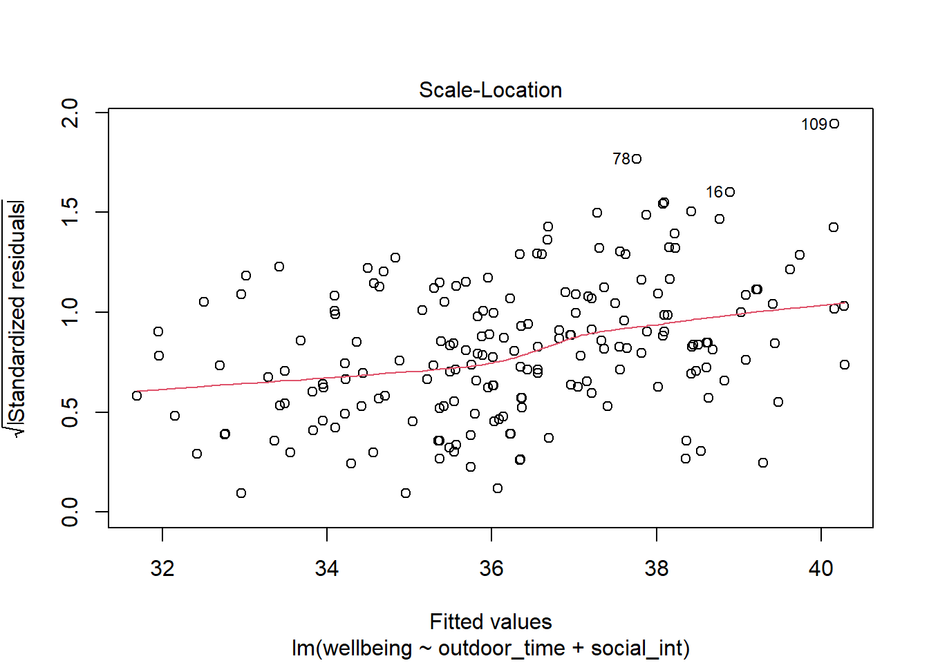
Quick Tip if plotting using plot(model)
As the residuals can be positive or negative, we can make it easier to assess equal spread by improving the ‘resolution’ of the points.
We can make all residuals positive by discarding the sign (take the absolute value), and then take the square root to make them closer to each other.
A plot of \(\sqrt{|\text{Standardized residuals}|}\) against the fitted values can be obtained via plot(model, which = 3).
Question 4
Assess whether there is autocorrelation in the error terms.
Write a sentence summarising whether or not you consider the assumption of independence to have been met (you may have to assume certain aspects of the study design).
Hint
Review the independence (of errors) flashcard.
Question 5
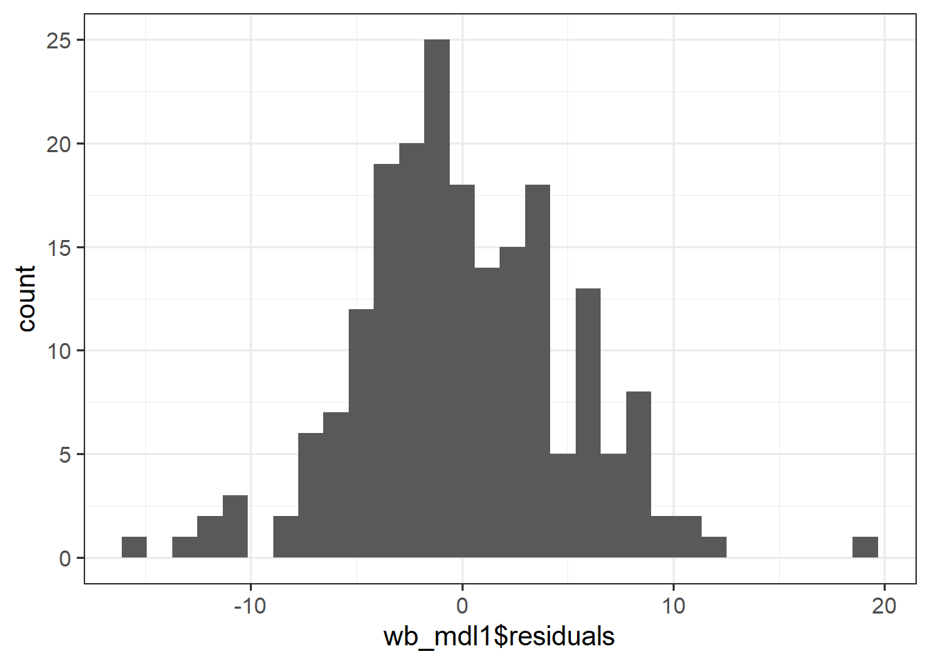
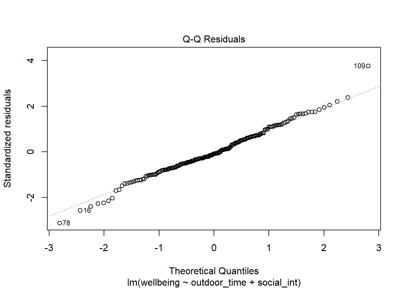
Check if the fitted model wb_mdl1 satisfies the normality assumption.
Write a sentence summarising whether or not you consider the assumption to have been met. Justify your answer with reference to the plots.
Hint
For more information, as well as tips to aid your interpretation, review the normality (of errors) flashcard.
Multicollinearity
Question 6
For wb_mdl1, calculate the variance inflation factor (VIF) for the predictors in the model.
Write a sentence summarising whether or not you consider multicollinearity to be a problem here.
Hint
For more information, as well as tips to aid your interpretation, review the multicollinearity flashcard.
Diagnostics
Question 7
Create a new tibble which contains:
- The original variables from the model (Hint, what does
wb_mdl1$modelgive you?) - The fitted values from the model \(\hat y\)
- The residuals \(\hat \epsilon\)
- The studentised residuals
- The hat values
- The Cook’s Distance values
Hint
For following will likely be useful to consider when creating your tibble():
- Think about what
wb_mdl1$modelgives you fitted()residuals()rstudent()hatvalues()cooks.distance()
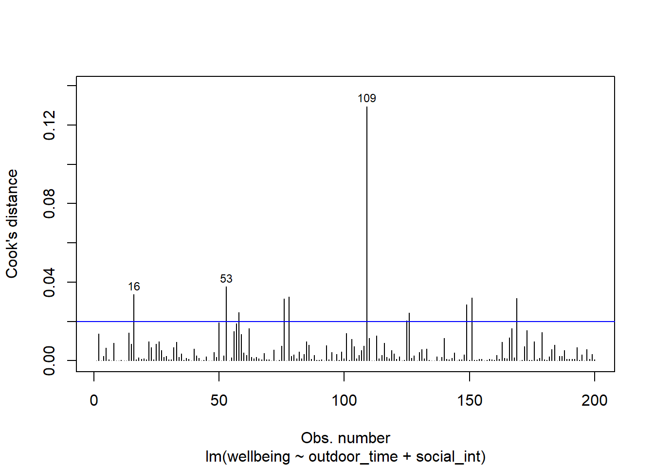
Question 8
From the tibble above, comment on the following:
- Looking at the studentised residuals, are there any outliers?
- Looking at the hat values, are there any observations with high leverage?
- Looking at the Cook’s Distance values, are there any highly influential points?
Hint
Alongside the lecture materials, review the individual case diagnostics flashcards and consider the commonly used cut-off criteria.
Question 9
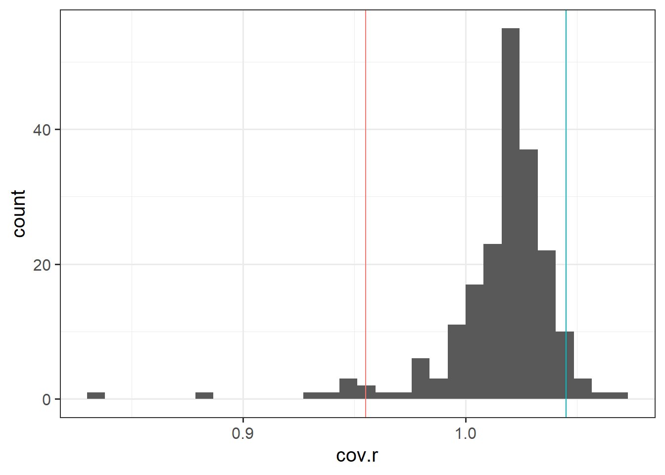
Use the function influence.measures() to extract these delete-1 measures1 of influence.
Choose a couple of these measures to focus on, exploring in more detail (you may want to examine values or even try plotting distributions).
Hint
Review the individual case diagnostics flashcards.
The function influence.measures() returns an infl-type object. To plot this, we need to find a way to extract the actual numbers from it.
What do you think names(influence.measures(wb_mdl1)) shows you? How can we use influence.measures(wb_mdl1)$<insert name here> to extract the matrix of numbers?
Question 10
What approaches would be appropriate to take given the issues highlighted above with the violations of assumptions and case diagnostic results?
Compile Report
Compile Report
Knit your report to PDF, and check over your work. To do so, you should make sure:
- Only the output you want your reader to see is visible (e.g., do you want to hide your code?)
- Check that the tinytex package is installed
- Ensure that the ‘yaml’ (bit at the very top of your document) looks something like this:
---
title: "this is my report title"
author: "B1234506"
date: "07/09/2024"
output: bookdown::pdf_document2
---
What to do if you cannot knit to PDF
If you are having issues knitting directly to PDF, try the following:
- Knit to HTML file
- Open your HTML in a web-browser (e.g. Chrome, Firefox)
- Print to PDF (Ctrl+P, then choose to save to PDF)
- Open file to check formatting
Hiding Code and/or Output
To not show the code of an R code chunk, and only show the output, write:
```{r, echo=FALSE}
# code goes here
```
To show the code of an R code chunk, but hide the output, write:
```{r, results='hide'}
# code goes here
```
To hide both code and output of an R code chunk, write:
```{r, include=FALSE}
# code goes here
```
Tinytex
You must make sure you have tinytex installed in R so that you can “Knit” your Rmd document to a PDF file:
install.packages("tinytex")
tinytex::install_tinytex()