| variable | description |
|---|---|
| id | Unique ID number |
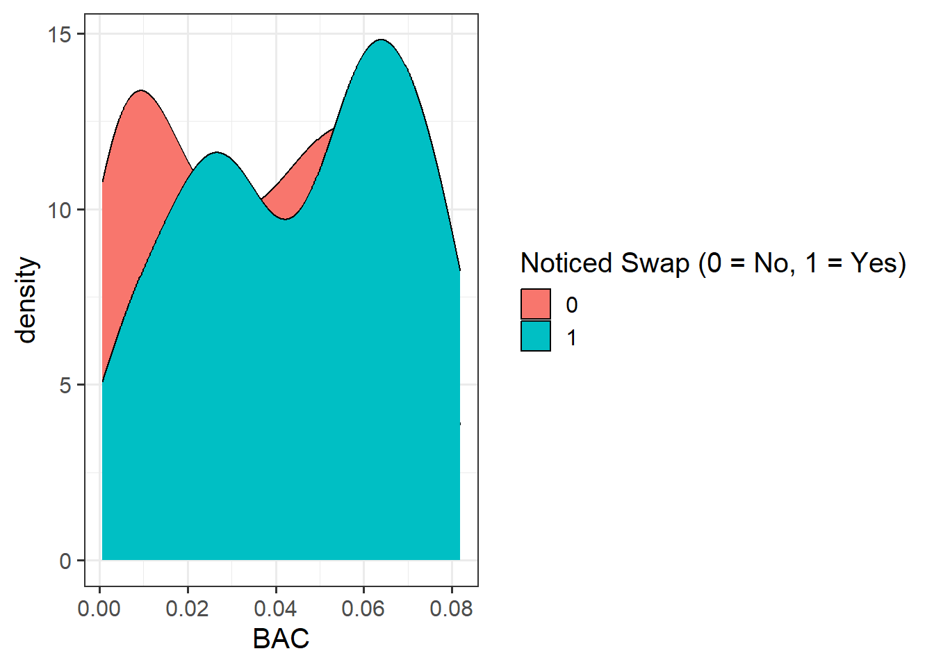
| bac | Blood Alcohol Content (BAC; %) - A BAC of 0.0 is sober, while in the United States 0.08 is legally intoxicated, and above that is very impaired. BAC levels above 0.40 are potentially fatal. |
| age | Age (in years) |
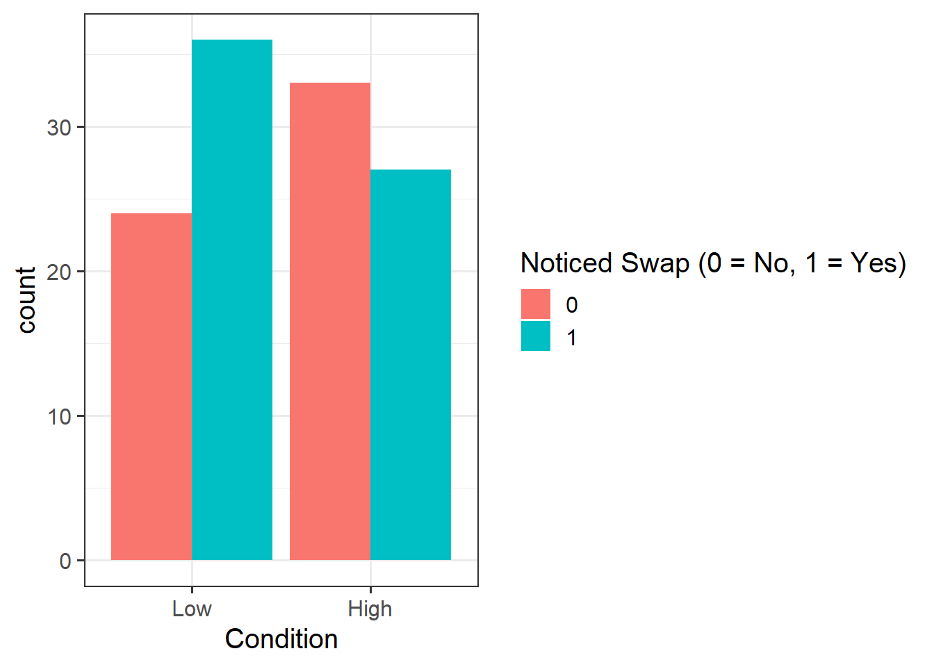
| condition | Perceptual load created by distracting object (door) and details and amount of papers handled in front of participant. Levels = Low, High |
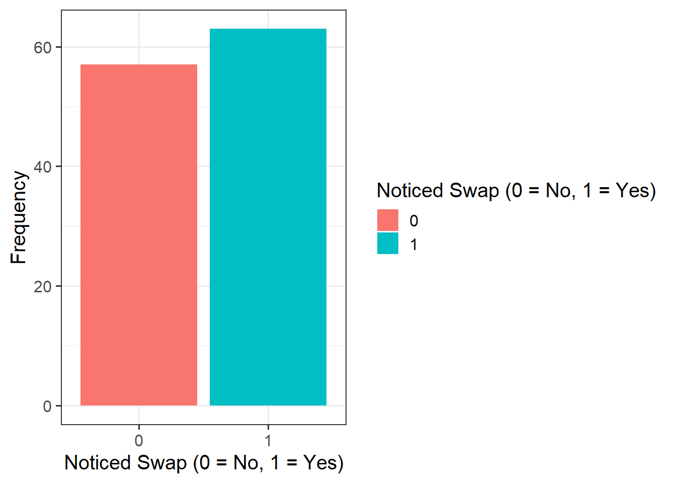
| notice | Whether or not the participant noticed the swap (No = 0 vs Yes = 1) |
Logistic Regression I
Learning Objectives
At the end of this lab, you will:
- Understand when to use a logistic model
- Understand how to fit and interpret a logistic model
What You Need
- Be up to date with lectures
Required R Packages
Remember to load all packages within a code chunk at the start of your RMarkdown file using library(). If you do not have a package and need to install, do so within the console using install.packages(" "). For further guidance on installing/updating packages, see Section C here.
For this lab, you will need to load the following package(s):
- tidyverse
- patchwork
- kableExtra
- psych
- sjPlot
Presenting Results
All results should be presented following APA guidelines.If you need a reminder on how to hide code, format tables/plots, etc., make sure to review the rmd bootcamp.
The example write-up sections included as part of the solutions are not perfect - they instead should give you a good example of what information you should include and how to structure this. Note that you must not copy any of the write-ups included below for future reports - if you do, you will be committing plagiarism, and this type of academic misconduct is taken very seriously by the University. You can find out more here.
Lab Data
You can download the data required for this lab here or read it in via this link https://uoepsy.github.io/data/drunkdoor.csv
Study Overview
Research Question
Is susceptibility to change blindness influenced by age, level of alcohol intoxication, and perceptual load?
Setup
Setup
- Create a new RMarkdown file
- Load the required package(s)
- Read the drunkdoor dataset into
R, assigning it to an object nameddrunkdoor
Exercises
Study & Analysis Plan Overview
Question 1
Firstly, examine the dataset, and perform any necessary and appropriate data management steps.
Next, think about the scales that the variables are currently on, with a particular focus on BAC, age, and condition. Consider:
- Do you want BAC on the current scale, or could you transform it somehow? Consider that instead of the coefficient representing the difference when moving from 0% to 1% BAC (1% blood alcohol is fatal!), we might want to have the difference associated with 0% to 0.01% BAC (i.e, a we want to talk about effects in terms of changing 1/100th of a percentage of BAC)
- Do you want age to be centred at 0 years (as it currently is), or could you re-centre to make it more meaningful?
- In your data management, you will hopefully make condition a factor, but have you considered the reference level? It would likely make most sense for this to be set as “Low”.
Hint
The
str()function will return the overall structure of the dataset, this can be quite handy to look at.When considering the scale of your BAC and age variables, review the data transformation flashcards.
Data Management
- Convert categorical variables to factors, and if needed, provide better variable names
- Label factors appropriately to aid with your model interpretations if required
- Check that the dataset is complete (i.e., are there any
NAvalues?). We can check this usingis.na()
Note that all of these steps can be done in combination - the mutate() and factor() functions will likely be useful here.
Question 2
Provide a brief overview of the study design and data, before detailing your analysis plan to address the research question.
Hint
- Give the reader some background on the context of the study
- State what type of analysis you will conduct in order to address the research question
- Specify the model to be fitted to address the research question (note that you will need to specify the reference level of your categorical variable)
- Specify your chosen significance (\(\alpha\)) level
- State your hypotheses
Much of the information required can be found in the Study Overview codebook.
Descriptive Statistics & Visualisations
Question 3
Provide a table of descriptive statistics and visualise your data.
Remember to interpret these in the context of the study.
Hint
Review the many ways to numerically and visually explore your data by reading over the data exploration flashcards.
For examples, see flashcards on descriptives statistics tables - categorical and numeric values examples.
Specifics to consider:
For your table of descriptive statistics, both the
group_by()andsummarise()functions will come in handy hereFor your visualisations, you will need to specify
as_factor()when plotting the notice variable since this is numeric, but we want it to be treated as a factor only for plotting purposes
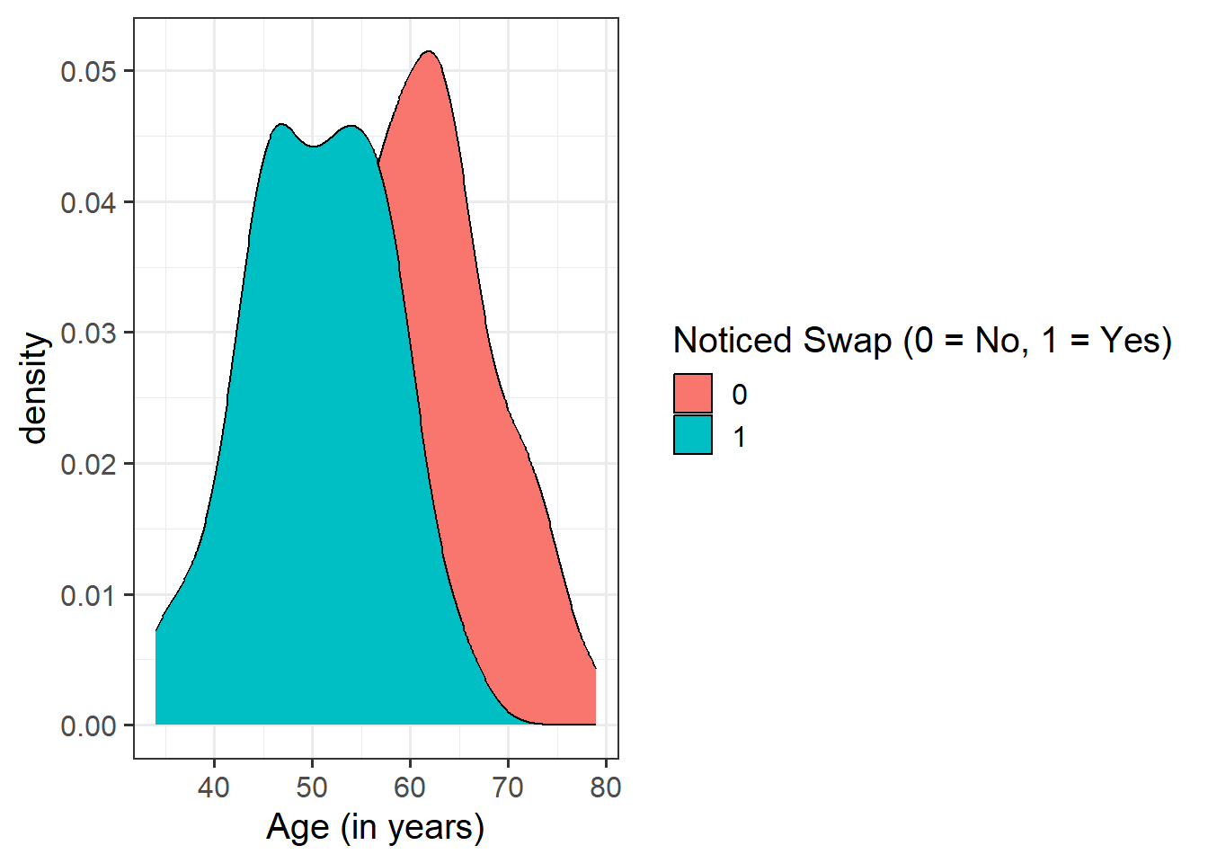
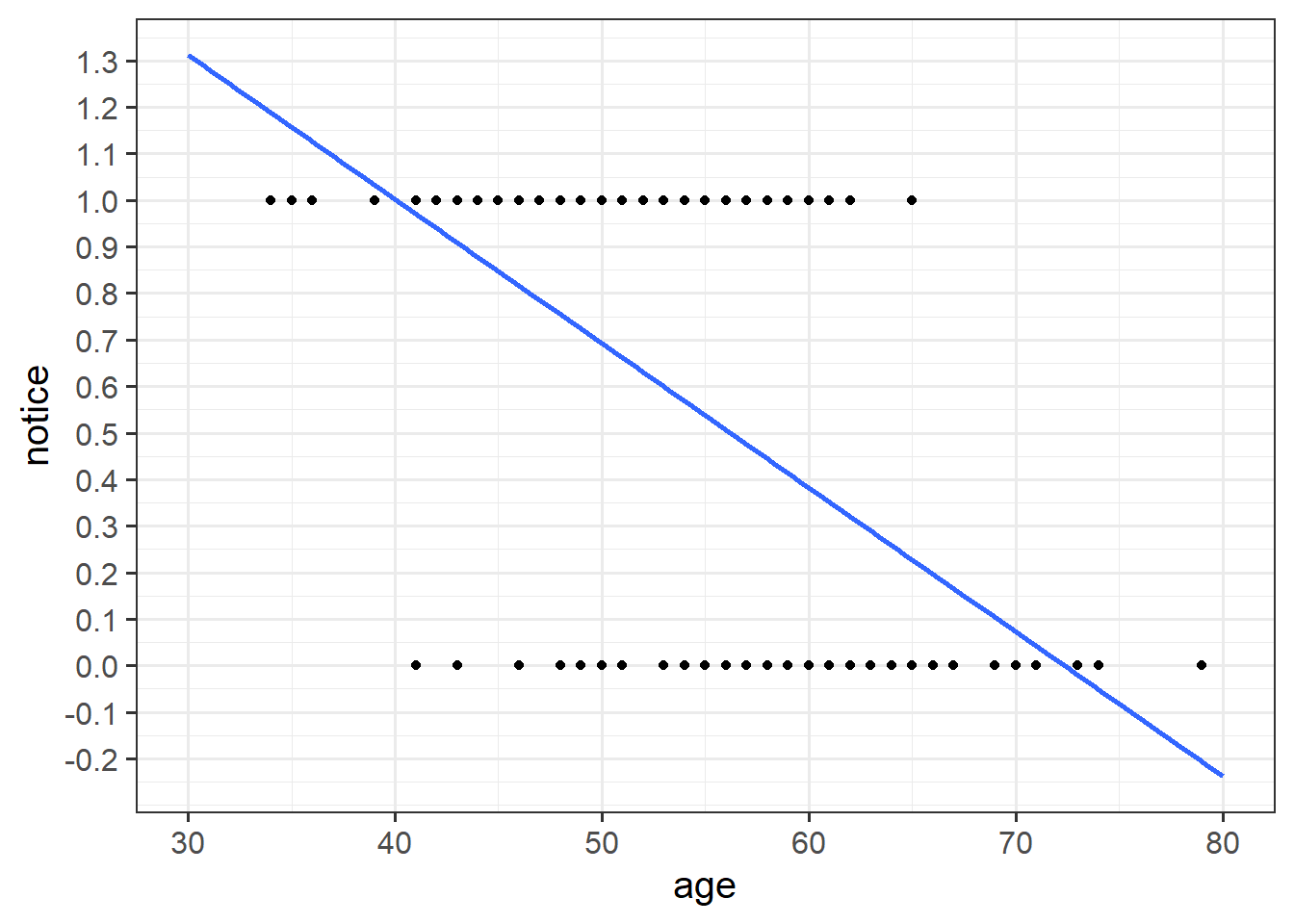
Question 4
For the moment, lets just consider the association between notice and age. Visually following the line from the plot produced below, what do you think the predicted model value would be for someone who is aged 30? What does this value mean?
Model Fitting & Interpretation
Question 5
Fit your model using glm(), and assign it as an object with the name “changeblind_mdl”.
Hint
For an overview of how to fit a binary logistic regression model using the glm() function, see the binary logistic regression flashcard.
For an example, review the binary logistic regression - example flashcard.
Question 6
Conduct a model comparison of your model above against the null model. Report the results of the model comparison in APA format.
Hint
Consider whether or not your models are nested. The model comparisons - logistic regression flashcards may be helpful to revisit.
Question 7
Interpret your coefficients in the context of the study. When doing so, it may be useful to translate the log-odds back into odds.
Hint
For an overview of how probability, odds, and log-odds are related, review the probability, odds, and log-odds flashcard.
If you need help interpreting coefficients, review the interpretation of coefficients flashcard.
For an example, review the binary logistic regression - example flashcard.
Visualise Model
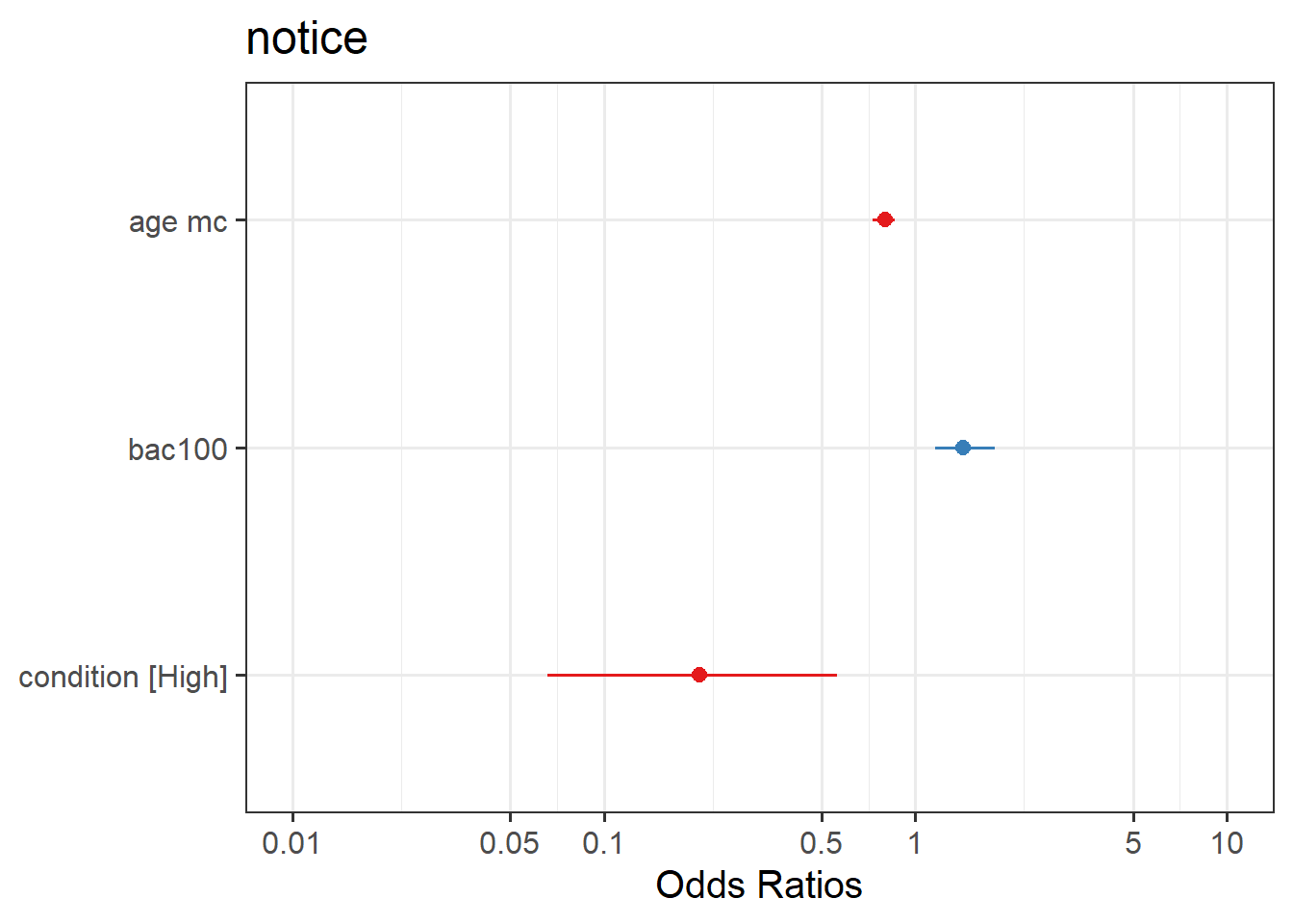
Question 8
Plot the predicted model estimates.
Hint
Here you will need to use plot_model() from the sjPlot package. To get your estimates, you will need to specify type = "est".
Writing Up & Presenting Results
Question 9
Provide key model results in a formatted table.
Hint
Use tab_model() from the sjPlot package. For a quick guide, review the tables flashcard.
Question 10
Interpret your results in the context of the research question and report your model in full.
Make reference to the regression table.
Hint
For an example of coefficient interpretation, review the interpretation of coefficients flashcard.
Compile Report
Compile Report
Knit your report to PDF, and check over your work. To do so, you should make sure:
- Only the output you want your reader to see is visible (e.g., do you want to hide your code?)
- Check that the tinytex package is installed
- Ensure that the ‘yaml’ (bit at the very top of your document) looks something like this:
---
title: "this is my report title"
author: "B1234506"
date: "07/09/2024"
output: bookdown::pdf_document2
---
What to do if you cannot knit to PDF
If you are having issues knitting directly to PDF, try the following:
- Knit to HTML file
- Open your HTML in a web-browser (e.g. Chrome, Firefox)
- Print to PDF (Ctrl+P, then choose to save to PDF)
- Open file to check formatting
Hiding Code and/or Output
To not show the code of an R code chunk, and only show the output, write:
```{r, echo=FALSE}
# code goes here
```
To show the code of an R code chunk, but hide the output, write:
```{r, results='hide'}
# code goes here
```
To hide both code and output of an R code chunk, write:
```{r, include=FALSE}
# code goes here
```
Tinytex
You must make sure you have tinytex installed in R so that you can “Knit” your Rmd document to a PDF file:
install.packages("tinytex")
tinytex::install_tinytex()