Interactions II: Num x Num

Learning Objectives

At the end of this lab, you will:

  1. Understand the concept of an interaction
  2. Be able to interpret the meaning of a numeric \(\times\) numeric interaction
  3. Understand the principle of marginality and why this impacts modelling choices with interactions
  4. Be able to visualize and probe interactions

What You Need

  1. Be up to date with lectures
  2. Have completed previous lab exercises from Week 1

Required R Packages

Remember to load all packages within a code chunk at the start of your RMarkdown file using library(). If you do not have a package and need to install, do so within the console using install.packages(" "). For further guidance on installing/updating packages, see Section C here.

For this lab, you will need to load the following package(s):

  • tidyverse
  • psych
  • sjPlot
  • kableExtra
  • sandwich
  • interactions

Presenting Results

All results should be presented following APA guidelines.If you need a reminder on how to hide code, format tables/plots, etc., make sure to review the rmd bootcamp.

The example write-up sections included as part of the solutions are not perfect - they instead should give you a good example of what information you should include and how to structure this. Note that you must not copy any of the write-ups included below for future reports - if you do, you will be committing plagiarism, and this type of academic misconduct is taken very seriously by the University. You can find out more here.

Lab Data

You can download the data required for this lab here or read it in via this link https://uoepsy.github.io/data/scs_study.csv

Study Overview

Research Question

Does the effect of social comparison on symptoms of depression, anxiety and stress vary depending on level of Neuroticism?

Social Comparison Study data codebook

Setup

Setup
  1. Create a new RMarkdown file
  2. Load the required package(s)
  3. Read the scs_study dataset into R, assigning it to an object named scs_study

#Loading the required package(s)
library(tidyverse)
library(psych)
library(sjPlot)
library(kableExtra) 
library(sandwich)
library(interactions)

#Reading in data and storing in object named 'scs_study'
scs_study <- read_csv("https://uoepsy.github.io/data/scs_study.csv")

Exercises

Study & Analysis Plan Overview

Question 1

Provide a brief overview of the study design and data, before detailing your analysis plan to address the research question.

  • Give the reader some background on the context of the study
  • State what type of analysis you will conduct in order to address the research question
  • Specify the model to be fitted to address the research question
  • Specify your chosen significance (\(\alpha\)) level
  • State your hypotheses

Much of the information required can be found in the Study Overview codebook.

The statistical models flashcards may also be useful to refer to. Specifically the interaction models flashcards and numeric x numeric example flashcards might be of most use.

The scs_study dataset contained information on 656 participants, including \(z\)-scores on 5 personality traits assessed by the Big-Five Aspects Scale (BFAS; Openness, Conscientiousness, Extraversion, Agreeableness and Neuroticism). Participants were also assessed on the Social Comparison Scale (SCS), which is an 11-item scale measuring self-perception (relative to others) of social rank, attractiveness and belonging, and the Depression Anxiety and Stress Scale (DASS-21) - a 21 item measure with higher scores indicating higher severity of symptoms. For both of these measures, only total scores were available. Items in the SCS were measured on a 5-point scale, giving minimum and maximum possible scores of 11 and 55 respectively. Items in the DASS-21 were measured on a 4-point scale, meaning that scores could range from 21 to 84.

Density plots and histograms will be used to visualise the marginal distributions of DASS-21 Scores, SCS Scores, and Neuroticism. To understand the strength of association among the variables, we will estimate the correlation coefficients; and to visualise these associations scatterplots will be used. To address the research question of whether Neuroticism moderated the effect of social comparison on depression and anxiety, we are going to fit the following interaction model:

\[ \begin{align} \text{DASS-21 Score} ~=~ & \beta_0 + \beta_1 \cdot \text{SCS Score} + \beta_2 \cdot \text{Neuroticism} \\ & + \beta_3 \cdot (\text{Neuroticism} \cdot \text{SCS Score}) + \epsilon \end{align} \] Effects will be considered statistically significant at \(\alpha=.05\)

Our hypotheses are:

\(H_0: \beta_3 = 0\)

The effect of social comparison on symptoms of depression, anxiety and stress does not vary depending on level of Neuroticism.

\(H_1: \beta_3 \neq 0\)

The effect of social comparison on symptoms of depression, anxiety and stress does vary depending on level of Neuroticism.

Descriptive Statistics & Visualisations

Question 2

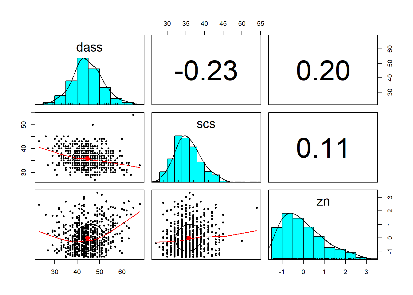
Provide a table of descriptive statistics and visualise your data. You may also want to consider estimating the associations among the variables of interest.

Remember to interpret these in the context of the study.

Review the many ways to numerically and visually explore your data by reading over the data exploration flashcards.

For examples, see flashcards on descriptives statistics tables - numeric values only examples and numeric x numeric example - visualise data.

The pairs.panels() function may come in handy here to complete multiple tasks at once!

Descriptive statistics presented in a well formatted table:

# note that we are selecting only our three variables of interest (dass, scs, zn)

scs_study %>%
    select(dass, scs, zn) %>% 
    describe() %>%
    kable(caption = "Descriptive Statistics - DASS-21, SCS, and Neuroticism (Z-Scored)", digits = 2) %>%
    kable_styling()
Table 1: Descriptive Statistics - DASS-21, SCS, and Neuroticism (Z-Scored)
Descriptive Statistics - DASS-21, SCS, and Neuroticism (Z-Scored)
vars n mean sd median trimmed mad min max range skew kurtosis se
dass 1 656 44.72 6.76 44.00 44.62 5.93 23.00 68.00 45.0 0.18 0.33 0.26
scs 2 656 35.77 3.53 35.00 35.59 2.97 27.00 54.00 27.0 0.60 0.96 0.14
zn 3 656 0.00 1.00 -0.21 -0.10 1.00 -1.45 3.35 4.8 0.80 0.04 0.04

Visualise associations among variables of interest:

scs_study %>% 
  select(dass, scs, zn) %>%
  pairs.panels()

Description of individual variables:

  • The marginal distribution of scores on the Depression, Anxiety and Stress Scale (DASS-21) was unimodal with a mean of 44.72 and a standard deviation of 6.76.
  • The marginal distribution of scores on the Social Comparison Scale (SCS) was unimodal with a mean of 35.77 and a standard deviation of 3.53.
  • The marginal distribution of Neuroticism (Z-scored) was positively skewed.

Description of correlations:

  • There was a weak, negative association between scores on the Depression Anxiety and Stress Scale and scores on the Social Comparison Scale for the participants in the sample \((r = -.23)\)
    • Severity of symptoms measured on the DASS-21 were lower, on average, for those who more favorably perceived their social rank
  • There was a weak, positive association between DASS-21 Scores and levels of Neuroticism \((r = .20)\)
    • Participants who were more neurotic tended to, on average, display a higher severity of symptoms of depression, anxiety and stress


Question 3

For demonstration purposes to help us visualise and understand the associations among our variables a little better, copy and run the two code chunks below. It takes the dataset, and uses the cut() function to add a new variable called “zn_group”, which is the “zn” variable split into 4 groups.

scs_study <-
  scs_study %>%
  mutate(
    zn_group = cut(zn, 4)
  )

We can see how it has split the “zn” variable by plotting the two against one another (note that the levels of the new variable are named according to the cut-points):

ggplot(data = scs_study, aes(x = zn_group, y = zn)) + 
  geom_point()

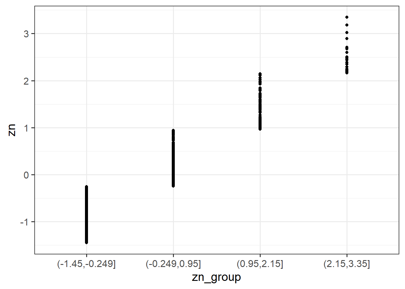
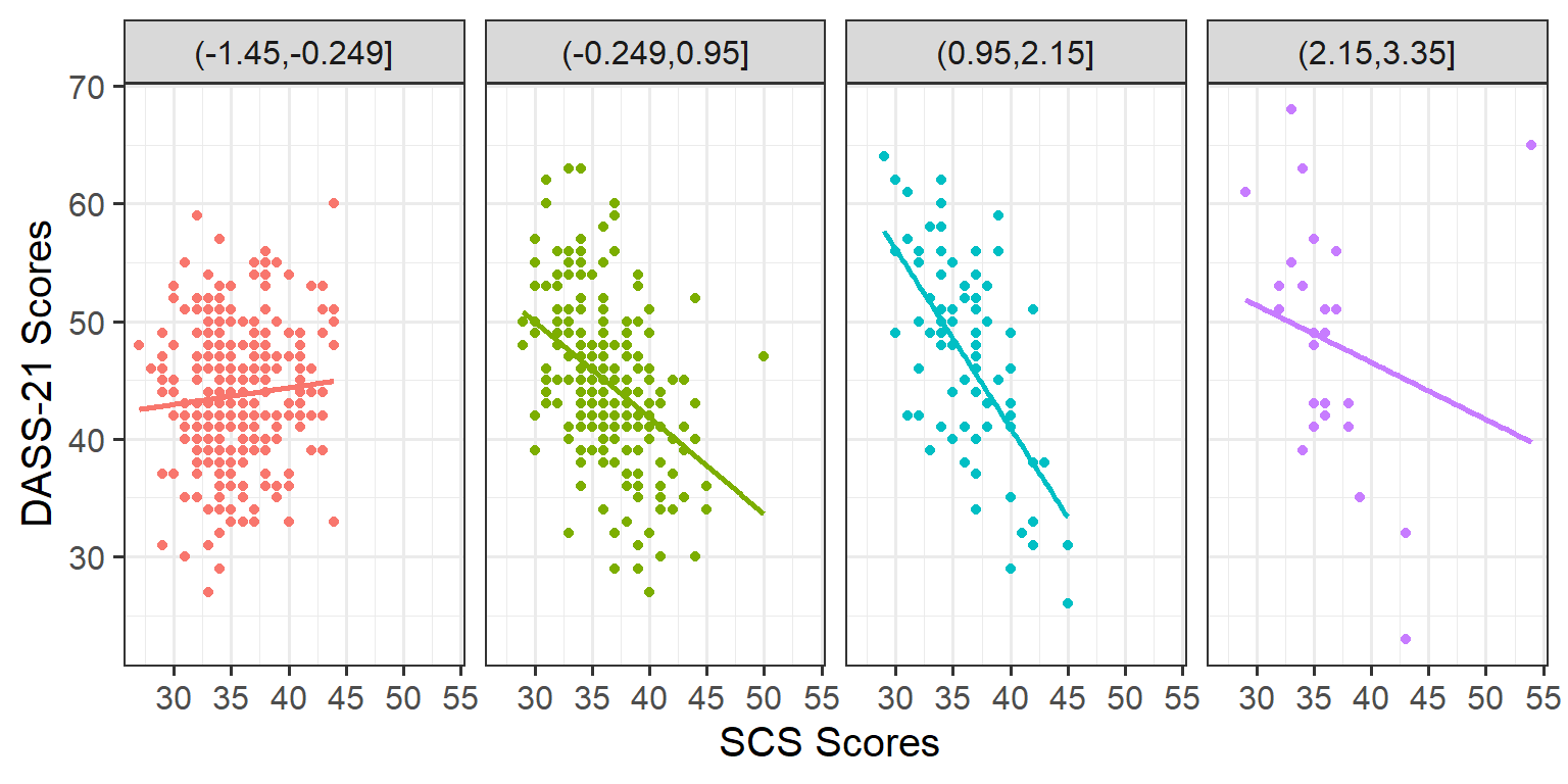
Plot the association between scores on the SCS and scores on the DASS-21, for each group of the variable we just created.

How does the pattern differ across groups? Does it suggest an interaction?

Rather than creating four separate plots, you might want to map some feature of the plot to the variable we created in the data, or make use of facet_wrap() / facet_grid().

Remember that you can specify geom_smooth() to add a trend line. For a recap, review the facet examples contained within the visual exploration flashcards. Alternatively, review the numeric x numeric example - visualise data flashcard.

ggplot(data = scs_study, aes(x = scs, y = dass, col = zn_group)) + 
  geom_point() + 
  geom_smooth(method='lm', se = FALSE) +
  facet_grid(~zn_group) +
  labs(x = "SCS Scores ", y = "DASS-21 Scores") +
  theme(legend.position = "none") # removes the legend

The association between DASS-21 scores and SCS scores appears to be different across these groups. For those with a relatively high Neuroticism score, the association seems stronger, while for those with a low Neuroticism score there is almost no discernible association.

This does suggest an interaction - the association of DASS-21 ~ SCS differed across the values of Neuroticism.


Visualising Interaction Terms

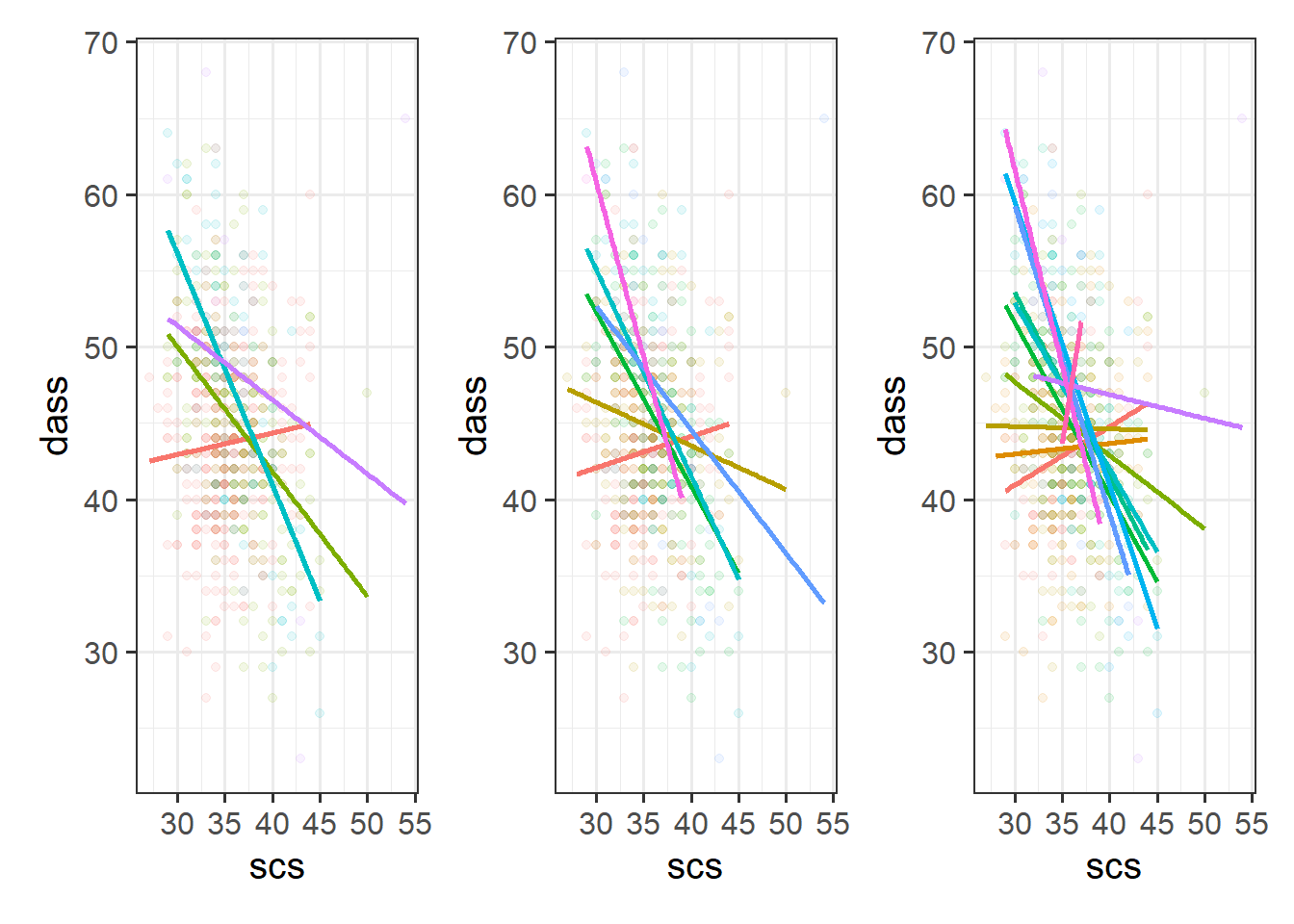
Cutting one of the explanatory variables up into groups essentially turns a numeric variable into a categorical one. We did this just to make it easier to visualise how an association differs across the values of another variable, because we can imagine a separate line for the association between SCS and DASS-21 scores for each of the groups of Neuroticism. However, in grouping a numeric variable like this we lose information. Neuroticism is measured on a continuous scale, and we want to capture how the association between SCS and DASS-21 differs across that continuum (rather than cutting it into chunks).

We could imagine cutting it into more and more chunks (see Figure 1), until what we end up with is an infinite number of lines - i.e., a three-dimensional plane/surface (recall that in for a multiple regression model with 2 explanatory variables, we can think of the model as having three-dimensions). The inclusion of the interaction term simply results in this surface no longer being necessarily flat. You can see this in Figure 2.

Figure 1: Separate regression lines DASS ~ SCS for Neuroticism when cut into 4 (left) or 6 (center) or 12 (right) groups.
Figure 2: 3D plot of regression surface with interaction. You can explore the plot in the figure below from different angles by moving it around with your mouse.

Model Fitting & Interpretation

Question 4

Consider that Neuroticism has already been \(z\)-scored, but scs has not. To ensure that we can compare the effects of our estimates (and so they are both on meaningful scales), standardize the scs variable.

Review the standardisation flashcards for a recap if needed. Note, it would be best to create a new z-scored variable to then use within the model in this instance.

# standardize scs score
scs_study <- 
  scs_study %>% 
    mutate(
      zscs = (scs-mean(scs))/sd(scs)
    )


Question 5

Fit your model (including the standardized predictor variables) using lm(), and assign it the name “dass_mdl”.

We can fit interaction models using the lm() function.

For an overview, see the interaction models flashcards.

For an example, review the interaction models > numeric x numeric example > model building flashcards.

#fit interaction model
dass_mdl <- lm(dass ~  zn*zscs, data = scs_study)

#check model output
summary(dass_mdl)

Call:
lm(formula = dass ~ zn * zscs, data = scs_study)

Residuals:
    Min      1Q  Median      3Q     Max 
-16.301  -3.825  -0.173   3.733  45.777 

Coefficients:
            Estimate Std. Error t value Pr(>|t|)    
(Intercept)  44.9324     0.2405 186.807  < 2e-16 ***
zn            1.5798     0.2409   6.559 1.11e-10 ***
zscs         -1.5691     0.2416  -6.495 1.64e-10 ***
zn:zscs      -1.8332     0.2316  -7.915 1.06e-14 ***
---
Signif. codes:  0 '***' 0.001 '**' 0.01 '*' 0.05 '.' 0.1 ' ' 1

Residual standard error: 6.123 on 652 degrees of freedom
Multiple R-squared:  0.1825,    Adjusted R-squared:  0.1787 
F-statistic:  48.5 on 3 and 652 DF,  p-value: < 2.2e-16


Question 6

Interpret your coefficients in the context of the study.

Recall that we can obtain our parameter estimates using various functions such as summary(),coef(), coefficients(), etc.

For an overview of how to interpret coefficients, review the interaction models > interpreting coefficients flashcard. It is important to remember that you have standardised the variables in your model, and this will affect your interpretation. For a recap on what standardisation is and how it affects the scales of your variables, review the standardisation flashcard.

For a specific example of coefficient interpretation, review the interaction models > numeric x numeric example > results interpretation flashcards.

Obtain parameter estimates:

coefficients(dass_mdl)
(Intercept)          zn        zscs     zn:zscs 
  44.932448    1.579769   -1.569097   -1.833169 

\(\beta_0\) = (Intercept) = 44.93

  • The intercept, or predicted DASS-21 score for an individual with an average SCS score and average Neuroticism score. In this case, the mean scores of SCS and Neuroticism are both 0 (since both have been standardised).
    • An individual with a Neuroticism score of 0 (\(Z\)-scored) and an SCS score of 0 (\(Z\)-scored) was expected to have a DASS-21 score of 44.93.

\(\beta_1\) = zn = 1.58

  • The simple slope of Neuroticism on DASS-21 scores with average SCS scores (0; \(Z\)-scored).
    • For an individual with an average SCS score (0; \(Z\)-scored), every 1 standard deviation increase in Neuroticism score was associated with a 1.58 point increase in DASS-21 scores.

\(\beta_2\) = zscs = -1.57

  • The simple slope of SCS scores on DASS-21 scores with average Neuroticism scores (0; \(Z\)-scored).
    • For an individual with an average Neuroticism score (0; \(Z\)-scored), every 1 standard deviation increase in SCS score was associated with a 1.57 decrease in DASS-21 scores.

\(\beta_3\) = zscs:zn = -1.83

  • The interaction between SCS score and Neuroticism on DASS-21 Scores - the change in the slope of SCS Scores as a function of Neuroticism.
    • For every 1 standard deviation increase in SCS scores, when Neuroticism scores increased by 1 standard deviation, the slope with DASS-21 scores was adjusted by -1.83.
    • The higher Neuroticism scores, the stronger the negative association between SCS Scores and DASS-21 scores - the association between SCS and DASS-21 scores became more negative by -1.83 points.

Visualise Interaction Model

Question 7

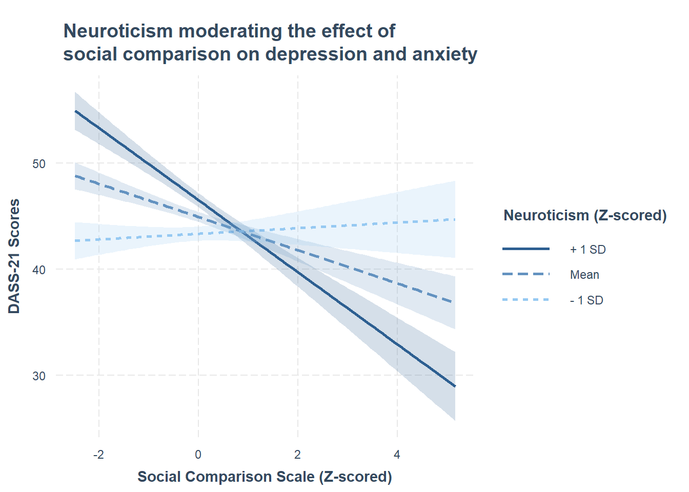
Using the probe_interaction() function from the interactions package, visualise the interaction effects from your model.

Try to summarise the interaction effects in a short and concise sentence.

plt_dass_mdl <- probe_interaction(model = dass_mdl, 
                  pred = zscs, 
                  modx = zn, 
                  cond.int = T,
                  interval = T, 
                  jnplot = T,
                  main.title = "Neuroticism moderating the effect of\nsocial comparison on depression and anxiety",
                  x.label = "Social Comparison Scale (Z-scored)",
                  y.label = "DASS-21 Scores",
                  legend.main = "Neuroticism (Z-scored)")

Let’s look at the plot - to do so you need to call interactplot from your object plt_dass_mdl:

plt_dass_mdl$interactplot
Figure 3: Simple Slopes for +/- 1 SD and Mean Neuroticism Scores

Recall that higher DASS-21 scores indicate higher severity of symptoms. Based on this, we can state:

  • For individuals 1 SD below the sample mean on Neuroticism, as their SCS Score increases, it appears that their DASS-21 scores remain flat / there is a very slight increase (i.e., their wellbeing do not change much)
  • For individuals with average levels of Neuroticism, as their SCS Score increases, it appears that their DASS-21 scores decreases (i.e., their wellbeing increases)
  • For individuals 1 SD above the sample mean on Neuroticism, as their SCS Score increases, it appears that their DASS-21 scores more steeply decreases (i.e., their wellbeing increases)


Question 8

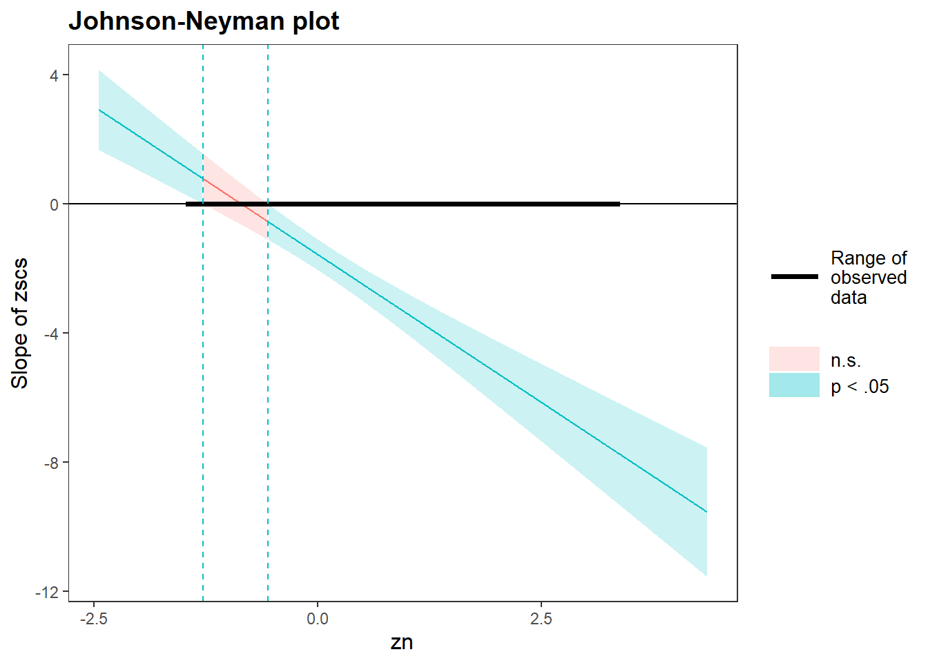
Conduct a simple slopes and regions of significance analysis.

For an overview and example, review the interaction models > numeric x numeric example > model visualisation flashcards. Pay particular attention to how you can extract specific parts of output.

plt_dass_mdl$simslopes
JOHNSON-NEYMAN INTERVAL

When zn is OUTSIDE the interval [-1.28, -0.55], the slope of zscs is p <
.05.

Note: The range of observed values of zn is [-1.45, 3.35]
SIMPLE SLOPES ANALYSIS

When zn = -1.000000e+00 (- 1 SD): 

                               Est.   S.E.   t val.      p
--------------------------- ------- ------ -------- ------
Slope of zscs                  0.26   0.35     0.76   0.45
Conditional intercept         43.35   0.34   127.47   0.00

When zn = -8.610271e-16 (Mean): 

                               Est.   S.E.   t val.      p
--------------------------- ------- ------ -------- ------
Slope of zscs                 -1.57   0.24    -6.50   0.00
Conditional intercept         44.93   0.24   186.81   0.00

When zn =  1.000000e+00 (+ 1 SD): 

                               Est.   S.E.   t val.      p
--------------------------- ------- ------ -------- ------
Slope of zscs                 -3.40   0.32   -10.59   0.00
Conditional intercept         46.51   0.34   136.52   0.00
Figure 4: Johnson-Neyman Plot

The Johnson-Neyman technique (see Figure 4) indicated that the association between DASS-21 scores and SCS was significant when Neuroticism scores were less than 1.28 standard deviations below the mean or greater than -0.55 standard deviations above the mean.

Writing Up & Presenting Results

Question 9

Provide key model results in a formatted table.

Use tab_model() from the sjPlot package. For a quick guide, review the tables flashcard.

#create table for results
tab_model(dass_mdl,
          dv.labels = "DASS-21 Scores",
          pred.labels = c("zscs" = "Social Comparison Scale (Z-scored)",
                          "zn" = "Neuroticism (Z-scored)",
                          "zscs:zn" = "Social Comparison Scale (Z-scored): Neutoricism (Z-scored)"),
          title = "Regression Table for DASS-21 Model")
Table 2: Regression table for DASS-21 model
Regression Table for DASS-21 Model
  DASS-21 Scores
Predictors Estimates CI p
(Intercept) 44.93 44.46 – 45.40 <0.001
Neuroticism (Z-scored) 1.58 1.11 – 2.05 <0.001
Social Comparison Scale
(Z-scored)
-1.57 -2.04 – -1.09 <0.001
zn:zscs -1.83 -2.29 – -1.38 <0.001
Observations 656
R2 / R2 adjusted 0.182 / 0.179


Question 10

Interpret your results in the context of the research question and report your model in full.

Make reference to the interaction plot and regression table.

For an example of coefficient interpretation, review the interaction models > numeric x numeric example > results interpretation flashcards.

Full regression results including 95% confidence intervals are shown in Table 2. The \(F\)-test for model utility was significant \((F(3,652) = 48.50, p<.001)\), and the model explained approximately 17.87% of the variability in DASS-21 scores.

There was a significant conditional association between DASS-21 Scores and SCS scores (\(Z\)-scored) \((\beta = -1.57, SE = 0.24, p < .001)\), suggesting that for those with Neuroticism scores of 0, DASS-21 scores decreased by 1.57 for every 1 standard deviation increase in SCS scores.

A significant conditional association was also evident between DASS-21 Scores and Neuroticism (\(Z\)-scored) \((\beta = 1.58, SE = 0.24, p <.001)\), suggesting that for those with SCS scores of 0, DASS-21 scores increased by 1.58 for every 1 standard deviation increase in Neuroticism.

The association between symptoms of depression and anxiety (DASS-21 scores) and social comparison was found to be dependent upon the level of Neuroticism, with a greater negative association between the two for those with higher levels of Neuroticism \((\beta = -1.83, SE = 0.23, p <.001)\). For every standard deviation increase in SCS Scores, the change in DASS-21 scores associated with an increase of 1 SD in Neuroticism was adjusted by -1.83. Thus, Neuroticism buffered the association between DASS-21 scores and SCS - this is visually displayed in Figure 3. We further used the Johnson-Neyman technique to probe the interaction, and to identify regions of significance. We identified that Neuroticism values (z-scored) outside the range of -1.28 to -0.55 were significant (see Figure 4).

Therefore, we have evidence to reject the null hypothesis (that the effect of social comparison on symptoms of depression, anxiety and stress does not vary depending on level of Neuroticism).

Compile Report

Compile Report

Knit your report to PDF, and check over your work. To do so, you should make sure:

  • Only the output you want your reader to see is visible (e.g., do you want to hide your code?)
  • Check that the tinytex package is installed
  • Ensure that the ‘yaml’ (bit at the very top of your document) looks something like this:
---
title: "this is my report title"
author: "B1234506"
date: "07/09/2024"
output: bookdown::pdf_document2
---

If you are having issues knitting directly to PDF, try the following:

  • Knit to HTML file
  • Open your HTML in a web-browser (e.g. Chrome, Firefox)
  • Print to PDF (Ctrl+P, then choose to save to PDF)
  • Open file to check formatting

To not show the code of an R code chunk, and only show the output, write:

```{r, echo=FALSE}
# code goes here
```

To show the code of an R code chunk, but hide the output, write:

```{r, results='hide'}
# code goes here
```

To hide both code and output of an R code chunk, write:

```{r, include=FALSE}
# code goes here
```

You must make sure you have tinytex installed in R so that you can “Knit” your Rmd document to a PDF file:

install.packages("tinytex")
tinytex::install_tinytex()

You should end up with a PDF file. If you have followed the above instructions and still have issues with knitting, speak with a Tutor.