Multiple Linear Regression

Learning Objectives

At the end of this lab, you will:

  1. Extend the ideas of single linear regression to consider regression models with two or more predictors
  2. Understand and interpret the coefficients in multiple linear regression models

Requirements

  1. Be up to date with lectures
  2. Have completed Week 1 lab exercises

Required R Packages

Remember to load all packages within a code chunk at the start of your RMarkdown file using library(). If you do not have a package and need to install, do so within the console using install.packages(" "). For further guidance on installing/updating packages, see Section C here.

For this lab, you will need to load the following package(s):

  • tidyverse
  • psych
  • patchwork
  • sjPlot
  • kableExtra

Presenting Results

All results should be presented following APA guidelines.If you need a reminder on how to hide code, format tables/plots, etc., make sure to review the rmd bootcamp.

The example write-up sections included as part of the solutions are not perfect - they instead should give you a good example of what information you should include and how to structure this. Note that you must not copy any of the write-ups included below for future reports - if you do, you will be committing plagiarism, and this type of academic misconduct is taken very seriously by the University. You can find out more here.

Lab Data

You can download the data required for this lab here or read it in via this link https://uoepsy.github.io/data/wellbeing_rural.csv

Study Overview

Research Question

Is there an association between wellbeing and time spent outdoors after taking into account the association between wellbeing and social interactions?

Wellbeing/Rurality data codebook.

Setup

Setup
  1. Create a new RMarkdown file
  2. Load the required package(s)
  3. Read the wellbeing dataset into R, assigning it to an object named mwdata

#Loading the required package(s)
library(tidyverse)
library(psych)
library(patchwork)
library(sjPlot)
library(kableExtra)

# Reading in data and storing to an object named 'mwdata'
mwdata <- read_csv("https://uoepsy.github.io/data/wellbeing_rural.csv")

Exercises

Study & Analysis Plan Overview

Question 1

Provide a brief overview of the study design and data, before detailing your analysis plan to address the research question.

  • Give the reader some background on the context of the study (you might be able to re-use some of the content you wrote for Lab 1 Q10 here)
  • State what type of analysis you will conduct in order to address the research question
  • Specify the model to be fitted to address the research question
  • Specify your chosen significance (\(\alpha\)) level
  • State your hypotheses

Much of the information required can be found in the Study Overview codebook. The statistical models flashcards may also be useful to refer to.

The mwdata dataset contained information on 200 hypothetical participants who lived in Edinburgh & Lothians area. Using a between-subjects design, the researchers collected information on participants’ wellbeing (measured via WEMWBS), outdoor time (hours per week), social interactions (number per week), routine (whether or not one was followed), location of residence (City, Suburb, or Rural), average weekly steps (in thousands), and age (in years).

Density plots and boxplots will be used to visualise the marginal distributions of wellbeing, social interactions, and outdoor time. To understand the strength of association among the variables, we will estimate the the correlation coefficients. To address the research question of whether there is an association between wellbeing and time spent outdoors after taking into account the association between wellbeing and social interactions, we are going to fit the following multiple linear regression model:

\[ \text{Wellbeing} = \beta_0 + \beta_1 \cdot \text{Social Interactions} + \beta_2 \cdot \text{Outdoor Time} + \epsilon \]

Effects will be considered statistically significant at \(\alpha=.05\).

Our hypotheses are:

\(H_0: \beta_2 = 0\): There is no association between wellbeing and time spent outdoors after taking into account the association between wellbeing and social interactions

\(H_1: \beta_2 \neq 0\): There is an association between wellbeing and time spent outdoors after taking into account the association between wellbeing and social interactions

Descriptive Statistics & Visualisations

Question 2

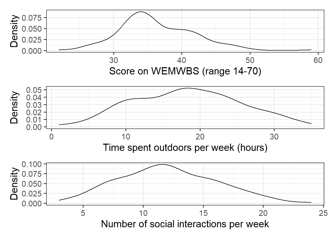
Alongside descriptive statistics, visualize the marginal distributions of the wellbeing, outdoor_time, and social_int variables.

Review the many ways to numerically and visually explore your data by reading over the data exploration flashcards.

For examples, see flashcards on descriptives statistics tables and data visualisation - marginal.
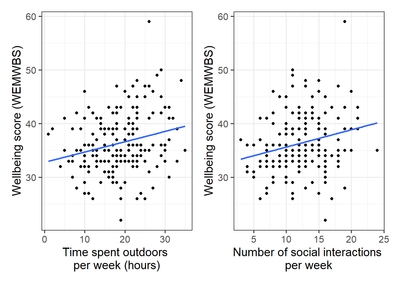
We can present our summary statistics for wellbeing, outdoor time, and social interactions as a well formatted table using kable():

mwdata %>% 
  select(wellbeing, outdoor_time, social_int) %>%
    describe() %>%
    kable(caption = "Wellbeing, Social Interactions, and Outdoor Time Descriptive Statistics", digits = 2) %>%
    kable_styling(full_width = FALSE)
Table 1: Wellbeing, Social Interactions, and Outdoor Time Descriptive Statistics
Wellbeing, Social Interactions, and Outdoor Time Descriptive Statistics
vars n mean sd median trimmed mad min max range skew kurtosis se
wellbeing 1 200 36.30 5.39 35 36.07 4.45 22 59 37 0.58 0.92 0.38
outdoor_time 2 200 18.25 7.10 18 18.14 7.41 1 35 34 0.06 -0.62 0.50
social_int 3 200 12.06 4.02 12 11.96 4.45 3 24 21 0.21 -0.40 0.28
  • The marginal distribution of scores on the WEMWBS was unimodal with a mean of approximately 36.3. There was variation in WEMWBS scores (SD = 5.39)
  • The marginal distribution of weekly hours spent outdoors was unimodal with a mean of approximately 18.25. There was variation in weekly hours spent outdoors (SD = 7.1)
  • The marginal distribution of numbers of social interactions per week was unimodal with a mean of approximately 12.06. There was variation in numbers of social interactions (SD = 4.02)

You should be familiar now with how to visualise a marginal distribution:

wellbeing_plot <- 
  ggplot(data = mwdata, aes(x = wellbeing)) +
  geom_density() +
  labs(x = "Score on WEMWBS (range 14-70)", y = "Density")

outdoortime_plot <- 
  ggplot(data = mwdata, aes(x = outdoor_time)) +
  geom_density() +
  labs(x = "Time spent outdoors per week (hours)", y = "Density")

social_plot <- 
  ggplot(data = mwdata, aes(x = social_int)) +
  geom_density() +
  labs(x = "Number of social interactions per week", y = "Density")

# arrange plots vertically 
wellbeing_plot / outdoortime_plot / social_plot
Figure 1: Marginal distribution plots of wellbeing sores, weekly hours spent outdoors, and social interactions


Question 3

Produce plots of the associations between the outcome variable (wellbeing) and each of the explanatory variables.

Review how to visually explore bivariate associations via the data visualisation flashcards.

For specifically visualising associations between variables, see the bivariate examples flashcards.

wellbeing_outdoor <- 
  ggplot(data = mwdata, aes(x = outdoor_time, y = wellbeing)) +
  geom_point() +
  geom_smooth(method = "lm", se = FALSE) + 
  labs(x = "Time spent outdoors \nper week (hours)", y = "Wellbeing score (WEMWBS)")

wellbeing_social <- 
  ggplot(data = mwdata, aes(x = social_int, y = wellbeing)) +
  geom_point() +
  geom_smooth(method = "lm", se = FALSE) + 
  labs(x = "Number of social interactions \nper week", y = "Wellbeing score (WEMWBS)")

# place plots adjacent to one another
wellbeing_outdoor | wellbeing_social
Figure 2: Scatterplots displaying the relationships between scores on the WEMWBS and a) weekly outdoor time (hours), and b) weekly number of social interactions

Both scatterplots indicated weak, positive, and linear associations both between wellbeing and outdoor time, and between wellbeing and the number of weekly social interactions.


Question 4

Produce a correlation matrix of the variables which are to be used in the analysis, and write a short paragraph describing the associations.

Review the correlation flashcards, and remember to interpret in the context of the research question.

We can either index the dataframe or select the variables of interest:

# correlation matrix of the three columns of interest (check which columns we need - in this case, 2,3, and 5)
round(cor(mwdata[,c(5,3,2)]), digits = 2)
             wellbeing social_int outdoor_time
wellbeing         1.00       0.24         0.25
social_int        0.24       1.00        -0.04
outdoor_time      0.25      -0.04         1.00
# select only the columns we want by variable name, and pass this to cor()
mwdata %>% 
  select(wellbeing, social_int, outdoor_time) %>%
  cor() %>%
  round(digits = 2)
             wellbeing social_int outdoor_time
wellbeing         1.00       0.24         0.25
social_int        0.24       1.00        -0.04
outdoor_time      0.25      -0.04         1.00
  • There was a weak, positive, linear association between WEMWBS scores and weekly outdoor time for the participants in the sample (\(r\) = .25). Higher number of hours spent outdoors each week was associated, on average, with higher wellbeing scores
  • There was a weak, positive, linear association between WEMWBS scores and the weekly number of social interactions for the participants in the sample (\(r\) = .24). More social interactions were associated, on average, with higher wellbeing scores
  • There was a negligible negative correlation between weekly outdoor time and the weekly number of social interactions (\(r\) = -.04)

Model Fitting & Interpretation

Question 5

Recall the model specified in Q1, and:

  1. State the parameters of the model. How do we denote parameter estimates?
  2. Fit the linear model in using lm(), assigning the output to an object called mdl1.

As we did for simple linear regression, we can fit our multiple regression model using the lm() function. For a recap, see the statistical models flashcards.

A model for the association between \(x_1\) = weekly numbers of social interactions, \(x_2\) = weekly outdoor time, and \(y\) = scores on the WEMWBS can be given by: \[ y = \beta_0 + \beta_1 x_1 + \beta_2 x_2 + \epsilon \\ \quad \\ \text{where} \quad \epsilon \sim N(0, \sigma) \text{ independently} \]

In the model specified above,

  • \(\mu_{y|x_1, x_2} = \beta_0 + \beta_1 x_1 + \beta_2 x_2\) represents the systematic part of the model giving the mean of \(y\) at each combination of values of \(x_1\) and \(x_2\);
  • \(\epsilon\) represents the error (deviation) from that mean, and the errors are independent from one another.

The parameters of our model are:

  • \(\beta_0\) (The intercept);
  • \(\beta_1\) (The slope across values of \(x_1\));
  • \(\beta_2\) (The slope across values of \(x_2\));
  • \(\sigma\) (The standard deviation of the errors).

When we estimate these parameters from the available data, we have a fitted model (recall that the h\(\hat{\textrm{a}}\)ts are used to distinguish our estimates from the true unknown parameters):

\[ \widehat{Wellbeing} = \hat \beta_0 + \hat \beta_1 \cdot Social~Interactions + \hat \beta_2 \cdot Outdoor~Time \] And we have residuals \(\hat \epsilon = y - \hat y\) which are the deviations from the observed values and our model-predicted responses.

Fitting the model in R:

mdl1 <- lm(wellbeing ~ social_int + outdoor_time, data = mwdata)


Additional Visual Explanation

Note that for simple linear regression we talked about our model as a line in 2 dimensions: the systematic part \(\beta_0 + \beta_1 x\) defined a line for \(\mu_y\) across the possible values of \(x\), with \(\epsilon\) as the random deviations from that line. But in multiple regression we have more than two variables making up our model.

In this particular case of three variables (one outcome + two explanatory), we can think of our model as a regression surface (see Figure 3). The systematic part of our model defines the surface across a range of possible values of both \(x_1\) and \(x_2\). Deviations from the surface are determined by the random error component, \(\hat \epsilon\).

Figure 3: Regression surface for wellbeing ~ social_int + outdoor_time, from two different angles

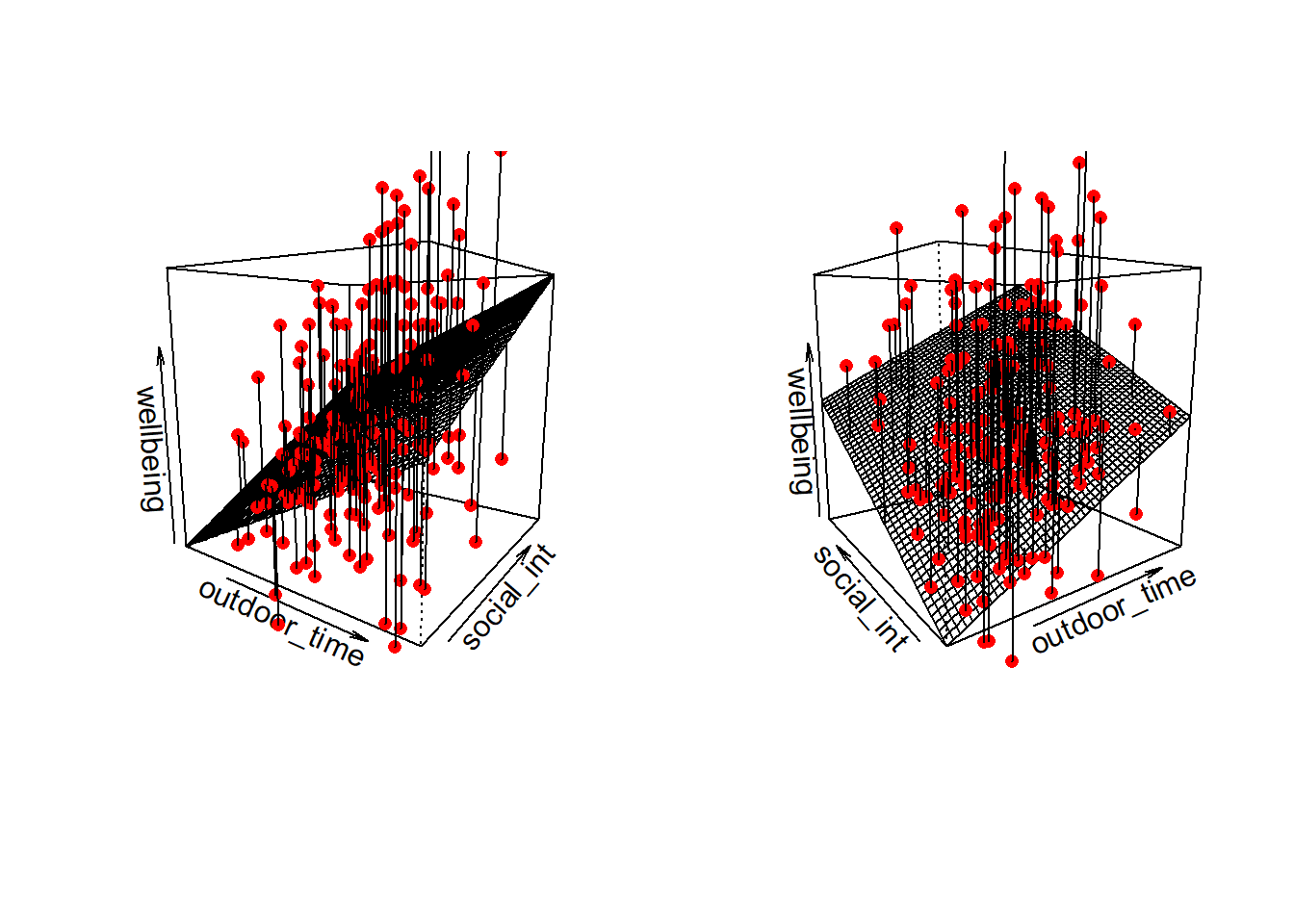
Don’t worry about trying to figure out how to visualise it if we had any more explanatory variables! We can only concieve of 3 spatial dimensions. One could imagine this surface changing over time, which would bring in a 4th dimension, but beyond that, it’s not worth trying!


Question 6

Using any of:

  • mdl1
  • mdl1$coefficients
  • coef(mdl1)
  • coefficients(mdl1)
  • summary(mdl1)

Write out the estimated parameter values of:

  1. \(\hat \beta_0\), the estimated average wellbeing score associated with zero hours of outdoor time and zero social interactions per week.
  2. \(\hat \beta_1\), the estimated increase in average wellbeing score associated with an additional social interaction per week (an increase of one), holding weekly outdoor time constant.
  3. \(\hat \beta_2\), the estimated increase in average wellbeing score associated with one hour increase in weekly outdoor time, holding the number of social interactions constant

To interpret and extract information, see the simple & multiple regression models - extracing information flashcards

mdl1$coefficients
 (Intercept)   social_int outdoor_time 
  28.6201808    0.3348821    0.1990943 
coef(mdl1)
 (Intercept)   social_int outdoor_time 
  28.6201808    0.3348821    0.1990943 
 (Intercept)   social_int outdoor_time 
  28.6201808    0.3348821    0.1990943 

Look under the “Estimate” column:

summary(mdl1)

Call:
lm(formula = wellbeing ~ social_int + outdoor_time, data = mwdata)

Residuals:
     Min       1Q   Median       3Q      Max 
-15.7611  -3.1308  -0.4213   3.3126  18.8406 

Coefficients:
             Estimate Std. Error t value Pr(>|t|)    
(Intercept)  28.62018    1.48786  19.236  < 2e-16 ***
social_int    0.33488    0.08929   3.751 0.000232 ***
outdoor_time  0.19909    0.05060   3.935 0.000115 ***
---
Signif. codes:  0 '***' 0.001 '**' 0.01 '*' 0.05 '.' 0.1 ' ' 1

Residual standard error: 5.065 on 197 degrees of freedom
Multiple R-squared:  0.1265,    Adjusted R-squared:  0.1176 
F-statistic: 14.26 on 2 and 197 DF,  p-value: 1.644e-06
  1. \(\hat \beta_0\) = 28.62
  2. \(\hat \beta_1\) = 0.33
  3. \(\hat \beta_2\) = 0.2


Question 7

Within what distance from the model predicted values (the regression line) would we expect 95% of WEMWBS wellbeing scores to be?

Either sigma() or part of the output from summary() will help you here. See Lab 1 Q5 for an example, or the simple & multiple regression models - extracting information flashcard.

sigma(mdl1)
[1] 5.065003

Look at the “Residual standard error” entry of the summary(mdl) output:

summary(mdl1)

Call:
lm(formula = wellbeing ~ social_int + outdoor_time, data = mwdata)

Residuals:
     Min       1Q   Median       3Q      Max 
-15.7611  -3.1308  -0.4213   3.3126  18.8406 

Coefficients:
             Estimate Std. Error t value Pr(>|t|)    
(Intercept)  28.62018    1.48786  19.236  < 2e-16 ***
social_int    0.33488    0.08929   3.751 0.000232 ***
outdoor_time  0.19909    0.05060   3.935 0.000115 ***
---
Signif. codes:  0 '***' 0.001 '**' 0.01 '*' 0.05 '.' 0.1 ' ' 1

Residual standard error: 5.065 on 197 degrees of freedom
Multiple R-squared:  0.1265,    Adjusted R-squared:  0.1176 
F-statistic: 14.26 on 2 and 197 DF,  p-value: 1.644e-06

The estimated standard deviation of the errors is \(\hat \sigma\) = 5.07. We would expect 95% of wellbeing scores to be within about 10.13 (\(2 \hat \sigma\)) from the model fit.


Question 8

Based on the model, predict the wellbeing scores for the following individuals who were not included in the original sample:

  • Leah: Social Interactions = 25; Outdoor Time = 3
  • Sean: Social Interactions = 19; Outdoor Time = 36
  • Mike: Social Interactions = 15; Outdoor Time = 20
  • Donna: Social Interactions = 7; Outdoor Time = 1

Who has the highest predicted wellbeing score, and who has the lowest?

First we need to pass the data into R:

wellbeing_query <- tibble(social_int = c(25, 19, 15, 7),
                          outdoor_time = c(3, 36, 20, 1))

And next use predict() to get their estimated wellbeing scores:

predict(mdl1, newdata = wellbeing_query)
       1        2        3        4 
37.58952 42.15034 37.62530 31.16345 

Sean has the highest predicted wellbeing score (42.15), and Donna the lowest (31.16).

Writing Up & Presenting Results

Question 9

Provide key model results in a formatted table.

Use tab_model() from the sjPlot package. For a quick guide, review the tables flashcard.

tab_model(mdl1,
          dv.labels = "Wellbeing (WEMWBS Scores)",
          pred.labels = c("social_int" = "Social Interactions (number per week)",
                          "outdoor_time" = "Outdoor Time (hours per week)"),
          title = "Regression Table for Wellbeing Model")
Table 2: Regression Table for Wellbeing Model
Regression Table for Wellbeing Model
  Wellbeing (WEMWBS Scores)
Predictors Estimates CI p
(Intercept) 28.62 25.69 – 31.55 <0.001
Social Interactions
(number per week)
0.33 0.16 – 0.51 <0.001
Outdoor Time (hours per
week)
0.20 0.10 – 0.30 <0.001
Observations 200
R2 / R2 adjusted 0.126 / 0.118


Question 10

Interpret your results in the context of the research question.

Make reference to the regression table.

Make sure to include a decision in relation to your null hypothesis - based on the evidence, should you reject or fail to reject the null?

From Figure 1, we can see that wellbeing \((M = 36.3, SD = 5.39)\), social interactions \((M = 12.06, SD = 4.02)\), and outdoor time \((M = 18.25, SD = 7.1)\) followed unimodal distributions. There were weak, positive, linear associations between WEMWBS scores and the weekly number of social interactions \((r = .24)\), and between WEMWBS scores and outdoor time \((r = .25)\) in the sample.

A multiple regression model was used to determine if there was an association between well-being and time spent outdoors after taking into account the association between well-being and social interactions. As presented in Table 2, outdoor time was significantly associated with wellbeing scores \((\beta = 0.20, SE = 0.05, p < .001)\) after controlling for the number of weekly social interactions. Results suggested that, holding constant social interactions, for every additional hour spent outdoors each week, wellbeing scores increased by 0.20 points. Therefore, we should reject the null hypothesis since \(p < .05\).

Compile Report

Compile Report

Knit your report to PDF, and check over your work. To do so, you should make sure:

  • Only the output you want your reader to see is visible (e.g., do you want to hide your code?)
  • Check that the tinytex package is installed
  • Ensure that the ‘yaml’ (bit at the very top of your document) looks something like this:
---
title: "this is my report title"
author: "B1234506"
date: "07/09/2024"
output: bookdown::pdf_document2
---

If you are having issues knitting directly to PDF, try the following:

  • Knit to HTML file
  • Open your HTML in a web-browser (e.g. Chrome, Firefox)
  • Print to PDF (Ctrl+P, then choose to save to PDF)
  • Open file to check formatting

Review Lesson 5 of the rmd bootcamp for a detailed description/worked examples.

To not show the code of an R code chunk, and only show the output, write:

```{r, echo=FALSE}
# code goes here
```

To show the code of an R code chunk, but hide the output, write:

```{r, results='hide'}
# code goes here
```

To hide both code and output of an R code chunk, write:

```{r, include=FALSE}
# code goes here
```

You must make sure you have tinytex installed in R so that you can “Knit” your Rmd document to a PDF file:

install.packages("tinytex")
tinytex::install_tinytex()

You should end up with a PDF file. If you have followed the above instructions and still have issues with knitting, speak with a Tutor.