Interactions III: Cat x Cat

Learning Objectives

At the end of this lab, you will:

Understand the concept of an interaction
Be able to interpret a categorical \(\times\) categorical interaction
Be able to visualize and probe interactions

What You Need

Be up to date with lectures
Have completed previous lab exercises from Week 1 and Week 2

Required R Packages

Remember to load all packages within a code chunk at the start of your RMarkdown file using library(). If you do not have a package and need to install, do so within the console using install.packages(" "). For further guidance on installing/updating packages, see Section C here.

For this lab, you will need to load the following package(s):

tidyverse
psych
sjPlot
kableExtra
sandwich
interactions

Presenting Results

All results should be presented following APA guidelines.If you need a reminder on how to hide code, format tables/plots, etc., make sure to review the rmd bootcamp.

The example write-up sections included as part of the solutions are not perfect - they instead should give you a good example of what information you should include and how to structure this. Note that you must not copy any of the write-ups included below for future reports - if you do, you will be committing plagiarism, and this type of academic misconduct is taken very seriously by the University. You can find out more here.

Lab Data

You can download the data required for this lab here or read it in via this link https://uoepsy.github.io/data/cognitive_experiment_3_by_2.csv

Study Overview

Research Question

Are there differences in types of memory deficits for those experiencing different cognitive impairment(s)?

Cognitive Exp 3x2 data codebook.

Description

A group of researchers wants to test a hypothesised theory according to which the difference in performance between explicit and implicit memory tasks will be greatest for Huntington patients in comparison to controls. On the other hand, the difference in performance between explicit and implicit memory tasks will not significantly differ between patients with amnesia in comparison to controls. The researchers designed a study yielding a 3 by 2 factorial design to test this theory.

The tasks chosen by the researchers have been picked to map onto the theoretical differences between the three types of research participants. The first task (grammar) is known to reflect implicit memory processes, whereas the recognition task is known to reflect explicit memory processes. If the theory is correct, we would expect the difference in scores between the recognition and grammar tasks to be relatively similar for the control and amnesiac groups, but relatively larger for the Huntingtons group compared to controls.

Keep in mind that each person has been randomly assigned to one of the two tasks, so there are five observations per cell of the design.¹

Data Dictionary

The data in cognitive_experiment_3_by_2.csv contain three attributes collected from \(n=30\) participants, and includes:

variable	description
Diagnosis	Diagnosis classifies the three types of individuals: 1 = Amnesic patients, 2 = Huntingtons patients, and 3 = Control group of individuals with no known neurological disorder
Task	Task tells us to which one of two tasks each study participant was randomly assigned to: 1 = Grammar (which consists of classifying letter sequences as either following or not following grammatical rules), and 2 = Recognition (which consists of recognising particular stimuli as stimuli that have previously been presented during the task)
Y	Score

Preview

The first six rows of the data are:

Diagnosis	Task	Y
1	1	44
1	1	63
1	1	76
1	1	72
1	1	45
1	2	70

Setup

Create a new RMarkdown file
Load the required package(s)
Read the cognitive_experiment_3_by_2 dataset into R, assigning it to an object named cog

Exercises

Study & Analysis Plan Overview

Question 1

Examine the dataset, and perform any necessary and appropriate data management steps.

Hint

The str() function will return the overall structure of the dataset, this can be quite handy to look at
Convert categorical variables to factors, and if needed, provide better variable names*
Label factors appropriately to aid with your model interpretations if required*
Check that the dataset is complete (i.e., are there any NA values?). We can check this using is.na()

Note that all of these steps can be done in combination - the mutate() and factor() functions will likely be useful here.

*See the numeric outcomes & categorical predictors flashcard.

Question 2

Choose appropriate reference levels for the Diagnosis and Task variables.

Hint

Read the Study Overview codebook carefully.

Review the specifying reference levels flashcard.

Question 3

Provide a brief overview of the study design and data, before detailing your analysis plan to address the research question.

Hint

Give the reader some background on the context of the study
State what type of analysis you will conduct in order to address the research question
Specify the model to be fitted to address the research question (note that you will need to specify the reference level of your categorical variable(s))
Specify your chosen significance (\(\alpha\)) level
State your hypotheses

Much of the information required can be found in the Study Overview codebook.

The statistical models flashcards may also be useful to refer to. Specifically the interaction models flashcards and categorical x categorical example flashcards might be of most use.

The cog dataset contained information on 30 hypothetical participants from a between-subjects study. Participants belonged to one of three ‘Diagnosis’ groups, which had 10 participants in each - Control, Amnesic, or Huntingtons. Participants from each of the Diagnosis groups were randomly assigned to one of two ‘Tasks’ to measure different memory processes - Grammar or Recognition. For the purpose of this analysis, ‘Control’ was designated as the reference group for Diagnosis, since it was the only group of participants with no known neurological disorder, and as there is no natural reference group for Diagnosis, we chose to leave this as ‘Grammar’.

Boxplots will be used to visualise the associations among Diagnosis and Task conditions. To address the research question of whether the difference in performance between explicit and implicit memory tasks will be greatest for Huntington patients in comparison to controls, we first need to define the dummy variables for both

Diagnosis:

\[ \begin{align} & D_\text{Amnesic} = \begin{cases} 1 & \text{if Diagnosis is Amnesic} \\ 0 & \text{otherwise} \end{cases} \quad \\ & D_\text{Huntingtons} = \begin{cases} 1 & \text{if Diagnosis is Huntingtons} \\ 0 & \text{otherwise} \end{cases} \quad \\ \\ & (\text{Control is base level}) \end{align} \]

and for Task:

\[ \begin{align} & \text{T}_\text{Recognition} = \begin{cases} 1 & \text{if Task is Recognition} \\ 0 & \text{otherwise} \end{cases} \quad \\ \\ & (\text{Grammar is base level}) \end{align} \]

Based on the above dummy coding, we are going to fit the following interaction model:

\[ \begin{aligned} \text{Score} &= \beta_0 \\ &+ \beta_1 \cdot \text{D}_\text{Amnesic} + \beta_2 \cdot \text{D}_\text{Huntingtons} \\ &+ \beta_3 \cdot \text{T}_\text{Recognition} \\ &+ \beta_4 \cdot (\text{D}_\text{Amnesic} \cdot \text{T}_\text{Recognition}) + \beta_5 \cdot (\text{D}_\text{Huntingtons} \cdot \text{T}_\text{Recognition}) \\ &+ \epsilon \end{aligned} \]

Effects will be considered statistically significant at \(\alpha=.05\)

Our hypotheses are:

\(H_0: \beta_5 = 0\)

The difference in performance between explicit and implicit memory tasks does not significantly differ between patients with Huntingtons in comparison to Controls.

\(H_1: \beta_5 \neq 0\)

The difference in performance between explicit and implicit memory tasks does significantly differ between patients with Huntingtons in comparison to Controls.

Descriptive Statistics & Visualisations

Question 4

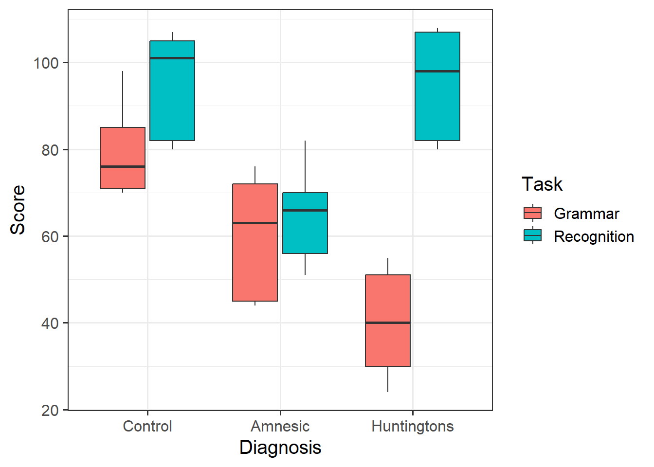
Provide a table of descriptive statistics and visualise your data.

Remember to interpret your plot in the context of the study.

Hint

Review the many ways to numerically and visually explore your data by reading over the data exploration flashcards.

For examples, see flashcards on descriptives statistics tables - categorical and numeric values examples and categorical x categorical example - visualise data.

Descriptive Statistics
Diagnosis	Task	M	SD	Min	Max
Control	Grammar	80	11.68	70	98
Control	Recognition	95	12.98	80	107
Amnesic	Grammar	60	14.92	44	76
Amnesic	Recognition	65	12.17	51	82
Huntingtons	Grammar	40	13.25	24	55
Huntingtons	Recognition	95	13.38	80	108

Model Fitting & Interpretation

Question 5

Fit the specified model using lm(), and assign it the name “cog_mdl”.

Hint

We can fit interaction models using the lm() function.

For an overview, see the interaction models flashcards.

For an example, review the interaction models > categorical x categorical example > model building flashcards.

Question 6

Recall your table of descriptive statistics - map each coefficient from the summary() output from “cog_mdl” to the group means.

Descriptive Statistics
Diagnosis	Task	M	SD	Min	Max
Control	Grammar	80	11.68	70	98
Control	Recognition	95	12.98	80	107
Amnesic	Grammar	60	14.92	44	76
Amnesic	Recognition	65	12.17	51	82
Huntingtons	Grammar	40	13.25	24	55
Huntingtons	Recognition	95	13.38	80	108

Coefficient	Value	Mapping to Group Means
\(\hat{\beta}_0\)	80	Mean(Control, Grammar)
\(\hat{\beta}_1\)	-20	Mean(Amnesic, Grammar) - Mean(Control, Grammar) = 60-80
\(\hat{\beta}_2\)	-40	Mean(Huntingtons, Grammar) - Mean(Control, Grammar) = 40-80
\(\hat{\beta}_3\)	15	Mean(Control, Recognition) - Mean(Control, Grammar) = 95-80
\(\hat{\beta}_4\)	-10	[Mean(Amnesic, Recognition) - Mean(Control, Recognition)] - [Mean(Amnesic, Grammar) - Mean(Control, Grammar)] = [65-95] - [60-80] = [-30] – [-20] = -10
\(\hat{\beta}_5\)	40	[Mean(Huntingtons, Recognition) - Mean(Control, Recognition)] - [Mean(Huntingtons, Grammar) - Mean(Control, Grammar)] = [95-95] - [40-80] = [0] – [-40] = 40

Question 7

Interpret your coefficients in the context of the study.

Hint

Recall that we can obtain our parameter estimates using various functions such as summary(),coef(), coefficients(), etc.

You may find it helpful to review your descriptive statistics from Q4, or the findings from your mapping exercise in Q6.

For an overview of how to interpret coefficients, review the interaction models > interpreting coefficients flashcard.

For a specific example of coefficient interpretation, review the interaction models > categorical x categorical example > results interpretation flashcards.

Obtain parameter estimates:

coefficients(cog_mdl)

                         (Intercept)                     DiagnosisAmnesic 
                                  80                                  -20 
                DiagnosisHuntingtons                      TaskRecognition 
                                 -40                                   15 
    DiagnosisAmnesic:TaskRecognition DiagnosisHuntingtons:TaskRecognition 
                                 -10                                   40

\(\beta_0\) = (Intercept) = 80

The intercept, or predicted scores for those in the Control diagnosis condition on the Grammar task.
- A Control participant completing the Grammar task was expected to score 80.

\(\beta_1\) = DiagnosisAmnesic = -20

The difference in scores between Amnesic and Control conditions on the Grammar task.
- When completing the Grammar task, individuals with Amnesia were estimated to score 20 points lower than Control participants.

\(\beta_2\) = DiagnosisHuntingtons = -40

The difference in score between Huntingtons and Control conditions on the Grammar task.
- When completing the Grammar task, individuals with Huntingtons were estimated to score 40 points lower than Control participants.

\(\beta_3\) = TaskRecognition = 15

The difference in score between individuals in the Control diagnosis condition completing Recognition and Grammar tasks
- Control participants were estimated to score 15 points higher when completing Recognition tasks in comparison to Grammar tasks.

\(\beta_4\) = DiagnosisAmnesic:TaskRecognition = -10

The difference in scores among those in Amnesia and Control diagnosis conditions between the Grammar and Recognition tasks
- The difference between scores for Amnesic and Control patients between Grammar and Recognition tasks differed by -10 points. The difference between Amnesics and controls was greater in the Recognition task, where in comparison to the Grammar task (where Amnesic were estimated to score 20 points lower than controls), there was an additional -10 difference between the two diagnosis groups.

\(\beta_5\) = DiagnosisHuntingtons:TaskRecognition = 40

The difference in scores among those in Huntingtons and Control diagnosis conditions between the Grammar and Recognition tasks
- The difference between scores for Huntingtons and Control patients between Grammar and Recognition tasks differed by 40 points. In comparison to the Grammar task (where Huntingtons patients were expected to score 40 points lower than controls), there was no difference between Huntingtons and controls in the Recognition task.

Visualise Interaction Model

Question 8

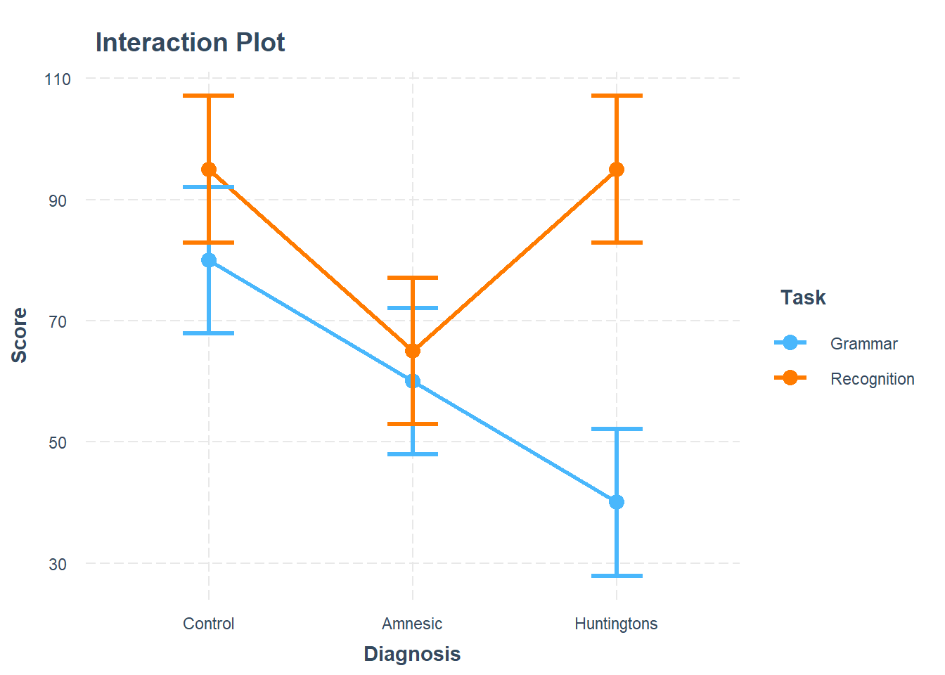
Using the cat_plot() function from the interactions package, visualise the interaction effects from your model.

Try to summarise the interaction effects in a few short and concise sentences.

Hint

For an overview and example, review the interaction models > categorical x categorical example > model visualisation flashcards.

Writing Up & Presenting Results

Question 9

Provide key model results in a formatted table.

Hint

Use tab_model() from the sjPlot package. For a quick guide, review the tables flashcard.

Regression Table for Scores Model
	Scores
Predictors	Estimates	CI	Statistic	p
(Intercept)	80.00	67.91 – 92.09	13.65	<0.001
Diagnosis [Amnesic]	-20.00	-37.10 – -2.90	-2.41	0.024
Diagnosis [Huntingtons]	-40.00	-57.10 – -22.90	-4.83	<0.001
Task [Recognition]	15.00	-2.10 – 32.10	1.81	0.083
Diagnosis [Amnesic] × Task [Recognition]	-10.00	-34.19 – 14.19	-0.85	0.402
Diagnosis [Huntingtons] × Task [Recognition]	40.00	15.81 – 64.19	3.41	0.002
Observations	30
R² / R² adjusted	0.739 / 0.685

Question 10

Interpret your results in the context of the research question and report your model in full.

Make reference to the interaction plot and regression table.

Hint

For an example of coefficient interpretation, review the interaction models > categorical x categorical example > results interpretation flashcards.

Compile Report

Knit your report to PDF, and check over your work. To do so, you should make sure:

Only the output you want your reader to see is visible (e.g., do you want to hide your code?)
Check that the tinytex package is installed
Ensure that the ‘yaml’ (bit at the very top of your document) looks something like this:

---
title: "this is my report title"
author: "B1234506"
date: "07/09/2024"
output: bookdown::pdf_document2
---

What to do if you cannot knit to PDF

If you are having issues knitting directly to PDF, try the following:

Knit to HTML file
Open your HTML in a web-browser (e.g. Chrome, Firefox)
Print to PDF (Ctrl+P, then choose to save to PDF)
Open file to check formatting

Hiding Code and/or Output

To not show the code of an R code chunk, and only show the output, write:

```{r, echo=FALSE}
# code goes here
```

To show the code of an R code chunk, but hide the output, write:

```{r, results='hide'}
# code goes here
```

To hide both code and output of an R code chunk, write:

```{r, include=FALSE}
# code goes here
```

Tinytex

You must make sure you have tinytex installed in R so that you can “Knit” your Rmd document to a PDF file:

install.packages("tinytex")
tinytex::install_tinytex()

Footnotes

Some researchers may point out that a design where each person was assessed on both tasks might have been more efficient. However, the task factor in such design would then be within-subjects, meaning that the scores corresponding to the same person would be correlated. To analyse such design we will need a different method which (spoiler alert!) will be discussed next year in DAPR3.↩︎