Simple Effects, Pairwise Comparisons, & Corrections

Learning Objectives

At the end of this lab, you will:

1. Understand how to interpret simple effects for experimental designs
2. Understand how to conduct pairwise comparisons
3. Understand how to apply corrections available for multiple comparisons

What You Need

1. Be up to date with lectures
2. Have completed previous lab exercises from Semester 1 Week 7, Semester 1 Week 8, Semester 1 Week 11, Semester 2 Week 1, Semester 2 Week 2, and Semester 2 Week 3.

Required R Packages

Remember to load all packages within a code chunk at the start of your RMarkdown file using library(). If you do not have a package and need to install, do so within the console using install.packages(" "). For further guidance on installing/updating packages, see Section C here.

For this lab, you will need to load the following package(s):

• tidyverse
• psych
• kableExtra
• sjPlot
• interactions
• patchwork
• emmeans

Presenting Results

All results should be presented following APA guidelines.If you need a reminder on how to hide code, format tables/plots, etc., make sure to review the rmd bootcamp.

The example write-up sections included as part of the solutions are not perfect - they instead should give you a good example of what information you should include and how to structure this. Note that you must not copy any of the write-ups included below for future reports - if you do, you will be committing plagiarism, and this type of academic misconduct is taken very seriously by the University. You can find out more here.

Lab Data

You can download the data required for this lab here or read it in via this link https://uoepsy.github.io/data/cognitive_experiment.csv

Note, you have already worked with some of this data last week - see Semester 2 Week 3 lab, but we now have a third Task condition - Classification.

Study Overview

Research Question

Are there differences in types of memory deficits for those experiencing different cognitive impairment(s)?

In this week’s exercises, we will further explore questions such as:

• Does level \(i\) of the first factor have an effect on the response?
• Does level \(j\) of the second factor have an effect on the response?
• Is there a combined effect of level \(i\) of the first factor and level \(j\) of the second factor on the response? In other words, is there interaction of the two factors so that the combined effect is not simply the additive effect of level \(i\) of the first factor plus the effect of level \(j\) of the second factor?

Cognitive Exp 3x3 data codebook.

Description

The researchers designed a study yielding a \(3 \times 3\) factorial design to test whether there are differences in types of memory deficits for those experiencing different cognitive impairment(s).

The tasks chosen by the researchers have been picked to map onto the theoretical differences between the three types of research participants. The Grammar and Classification tasks are known to reflect implicit memory processes, whereas the recognition task is known to reflect explicit memory processes. If the theory is correct, we would expect the difference in scores between the recognition and grammar/classification tasks to be relatively similar for the control and amnesiac groups, but relatively larger for the Huntingtons group compared to controls.

Data Dictionary

The data in cognitive_experiment.csv contain three attributes collected from \(n=45\) participants, and includes:

variable	description
Diagnosis	Diagnosis classifies the three types of individuals: 1 = Amnesic patients, 2 = Huntingtons patients, and 3 = Control group of individuals with no known neurological disorder
Task	Task tells us to which one of three tasks each study participant was randomly assigned to: 1 = Grammar (which consists of classifying letter sequences as either following or not following grammatical rules), 2 = Classification (which consists of classifying stimuli into certain groupings, based on previously indicated information about the groups characteristics), and 3 = Recognition (which consists of recognising particular stimuli as stimuli that have previously been presented during the task)
Y	Score

Data Overview

We have data from the 45 participants (15 amnesiacs, 15 Huntington individuals, and 15 controls). Recall that study involves two factors, now with three levels each. For each combination of factor levels we have 5 observations:

	Task
Diagnosis	grammar	classification	recognition
amnesic	44, 63, 76, 72, 45	72, 66, 55, 82, 75	70, 51, 82, 66, 56
huntingtons	24, 30, 51, 55, 40	53, 59, 33, 37, 43	107, 80, 98, 82, 108
control	76, 98, 71, 70, 85	92, 65, 86, 67, 90	107, 80, 101, 82, 105

The five observations are assumed to come from a population having a specific mean. The population means corresponding to each combination of factor levels can be schematically written as:

\[ \begin{matrix} & & & \textbf{Task} & \\ & & (j=1) & (j=2) & (j=3) & \\ & & \text{ grammar} & \text{ classification} & \text{ recognition} \\ & (i=1)\text{ control} & \mu_{1,1} & \mu_{1,2} & \mu_{1,3} \\ \textbf{Diagnosis} & (i=2)\text{ amnesic} & \mu_{2,1} & \mu_{2,2} & \mu_{2,3} \\ & (i=3)\text{ huntingtons} & \mu_{3,1} & \mu_{3,2} & \mu_{3,3} \end{matrix} \]

Preview

The first six rows of the data are:

Diagnosis	Task	Y
1	1	44
1	1	63
1	1	76
1	1	72
1	1	45
1	2	72

Setup

Setup

1. Create a new RMarkdown file
2. Load the required package(s)
3. Read the cognitive_experiment dataset into R, assigning it to an object named cog

#load packages
library(tidyverse)
library(psych)
library(kableExtra)
library(emmeans)
library(sjPlot)
library(interactions)
library(patchwork)

#read in data
cog <- read_csv('https://uoepsy.github.io/data/cognitive_experiment.csv')

Exercises

Study & Analysis Plan Overview

Question 1

Firstly, examine the dataset, and perform any necessary and appropriate data management steps.

Next, consider what would be the most appropriate coding constraint to apply in order to best address the research question - i.e., are we interested in whether group X (e.g., Amnesic) differed from group Y (e.g., Huntingtons), or whether group X (e.g., Amnesic) differed from the grand mean?

Choose appropriate reference levels for the Diagnosis and Task variables based on your decision above.

Hint

Data Management

• The str() function will return the overall structure of the dataset, this can be quite handy to look at
  
• Convert categorical variables to factors, and if needed, provide better variable names*
  
• Label factors appropriately to aid with your model interpretations if required*
  
• Check that the dataset is complete (i.e., are there any NA values?). We can check this using is.na()

Note that all of these steps can be done in combination - the mutate() and factor() functions will likely be useful here.

Coding Constraints

• If you think you’d benefit from a refresher on coding constraints, it might be best to revisit the materials from Semester 1 Block 2 (especially the dummy vs effects coding flashcard).
  
• If you would like an overview of coding constraints in the context of interaction models, review the categorical x categorical example > coding constraints flashcard.

Reference Levels

• Review the specifying reference levels flashcard.

*See the numeric outcomes & categorical predictors flashcard.

Let’s have a look at the data to see what we’re working with - str() or head() are a good place to start - and then we should check for any missing data (NA values):

#first look at dataset structure
str(cog)

spc_tbl_ [45 × 3] (S3: spec_tbl_df/tbl_df/tbl/data.frame)
 $ Diagnosis: num [1:45] 1 1 1 1 1 1 1 1 1 1 ...
 $ Task     : num [1:45] 1 1 1 1 1 2 2 2 2 2 ...
 $ Y        : num [1:45] 44 63 76 72 45 72 66 55 82 75 ...
 - attr(*, "spec")=
  .. cols(
  ..   Diagnosis = col_double(),
  ..   Task = col_double(),
  ..   Y = col_double()
  .. )
 - attr(*, "problems")=<externalptr> 

#now lets look at top 6 rows (or the head) of the dataset
head(cog)

# A tibble: 6 × 3
  Diagnosis  Task     Y
      <dbl> <dbl> <dbl>
1         1     1    44
2         1     1    63
3         1     1    76
4         1     1    72
5         1     1    45
6         1     2    72

#check for NAs 
table(is.na(cog))

FALSE 
  135 

# there are none - all FALSE

Next, lets convert Diagnosis and Task into factors, making the labels of each factor level more meaningful. According to the data description, the encoding of the factor Diagnosis is: 1 = amnesic patients, 2 = Huntingtons patients, and 3 = control patients. The encoding for the factor Task is: 1 = grammar task, 2 = classification task, and 3 = recognition task.

cog <- cog %>%
    mutate(
        Diagnosis = factor(Diagnosis, 
                           levels = c(1, 2, 3),
                           labels = c('amnesic', 'huntingtons', 'control'),
                           ordered = FALSE),
        Task = factor(Task, 
                      levels = c(1, 2, 3),
                      labels = c('grammar', 'classification', 'recognition'),
                      ordered = FALSE)) %>%
    rename(Score = Y)

Since we are interested in comparing groups, we should use dummy coding. By default, R uses dummy coding, so we do not need to make any changes to the coding constraint.

However, for our reference groups, we’re likely to want it to be the Control group for Diagnosis, and recognition for Task:

cog$Diagnosis <- fct_relevel(cog$Diagnosis, "control")
cog$Task <- fct_relevel(cog$Task, "recognition")

Question 2

Provide a brief overview of the study design and data, before detailing your analysis plan to address the research question.

Hint

• Give the reader some background on the context of the study (you might be able to re-use some of the content you wrote for Semester 2 Week 3 lab here, but note that we now have an extra condition within Task)
• Outline data checks / data cleaning
• State what type of analysis you will conduct in order to address the research question
• Specify the model to be fitted to address the research question (note that you will need to specify the reference level of your categorical variables. This will be somewhat similar to last week, but with the addition of Classification in Task, our model will contain a different number of parameters)
• Specify your chosen significance (\(\alpha\)) level
• State your hypotheses

Much of the information required can be found in the Study Overview codebook.

The statistical models flashcards may also be useful to refer to. Specifically the interaction models flashcards and categorical x categorical example flashcards might be of most use.

The cog dataset contained information on 45 hypothetical participants from a between-subjects study. Participants belonged to one of three ‘Diagnosis’ groups, which had 15 participants in each - Control, Amnesic, or Huntingtons. Participants from each of the Diagnosis groups were equally and randomly assigned to one of three ‘Tasks’ to measure different memory processes - Grammar, Classification, or Recognition - the former two measuring implicit memory and the latter explicit. This resulted in 5 participants from each Diagnosis group in each of the three Task conditions.

All participant data was complete, and categorical variables were coded as factors. For the purpose of this analysis, ‘Control’ was designated as the reference group for Diagnosis, since it was the only group of participants with no known neurological disorder. For Task, the recognition task measures explicit memory whereas the other two measure implicit memory, so this was specified as the reference group.

Boxplots will be used to visualise the associations among Diagnosis and Task conditions. To address the research question of whether the difference in performance between explicit and implicit memory tasks will be greatest for Huntington patients in comparison to controls, we first need to define the dummy variables for both

Diagnosis:

\[ \begin{gather*} \text{D}_\text{Amnesic} = \begin{cases} 1 & \text{if Diagnosis is Amnesic}\\ 0 & \text{otherwise} \end{cases} \\ \\ \text{D}_\text{Huntingtons} = \begin{cases} 1 & \text{if Diagnosis is Huntingtons}\\ 0 & \text{otherwise} \end{cases} \quad \\ \\ (\text{Control is base level}) \end{gather*} \]

and for Task:

\[ \begin{gather*} \text{T}_\text{Grammar} = \begin{cases} 1 & \text{if Task is Grammar}\\ 0 & \text{otherwise}\\ \end{cases}\ \\ \\ \text{T}_\text{Classification} = \begin{cases} 1 & \text{if Task is Classification}\\ 0 & \text{otherwise}\\ \end{cases}\\\ \quad \\ \\ (\text{Recognition is base level})\\ \end{gather*} \]

Based on the above dummy coding, we are going to fit the following interaction model:

\[ \begin{align} \text{Interaction Model}: \text{Score} &= \beta_0 \\ &+ \beta_1 \cdot \text{D}_\text{Amnesic} + \beta_2 \cdot \text{D}_\text{Huntingtons} \\ &+ \beta_3 \cdot \text{T}_\text{Grammar} + \beta_4 \cdot \text{T}_\text{Classification} \\ &+ \beta_5 \cdot (\text{D}_\text{Amnesic} \cdot \text{T}_\text{Grammar}) \\ &+ \beta_6 \cdot (\text{D}_\text{Huntingtons} \cdot \text{T}_\text{Grammar}) \\ &+ \beta_7 \cdot (\text{D}_\text{Amnesic} \cdot \text{T}_\text{Classification}) \\ &+ \beta_8 \cdot (\text{D}_\text{Huntingtons} \cdot \text{T}_\text{Classification}) \\ &+ \epsilon \end{align} \]

Effects will be considered statistically significant at \(\alpha = .05\)

Our hypotheses are:

\(H_0:\) All \(\beta_j = 0\) (for \(j = 5, 6, 7, 8\))

There are no significant differences in performance between explicit and implicit memory tasks for patients with different cognitive impairment(s).

\(H_1:\) At least one \(\beta_j \neq 0\) (for \(j = 5, 6, 7, 8\))

There are significant differences in performance between explicit and implicit memory tasks for patients with different cognitive impairment(s).

Descriptive Statistics & Visualisations

Question 3

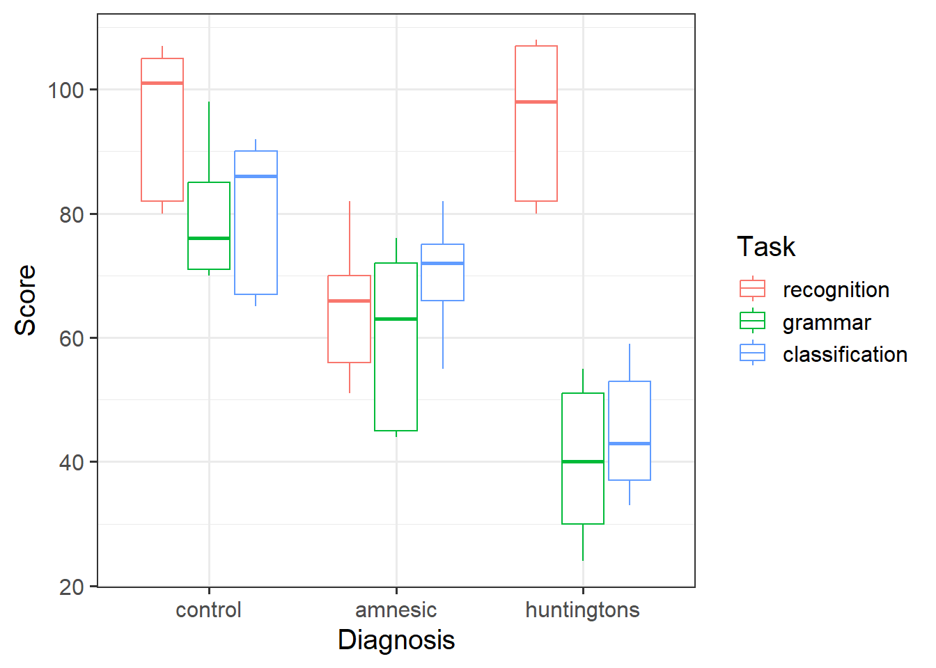
Provide a table of descriptive statistics and visualise your data.

Interpret the descriptive statistics and visualisations in the context of the study (i.e., comment on any observed differences among groups).

Hint

Review the many ways to numerically and visually explore your data by reading over the data exploration flashcards.

For examples, see flashcards on descriptives statistics tables - categorical and numeric values examples and categorical x categorical example - visualise data.

Make sure to comment on any observed differences among the sample means of the different conditions.

Numeric

Descriptive statistics presented in a well formatted table:

cog_stats <- cog %>% 
    group_by(Diagnosis, Task) %>%
    summarise(
        Mean = mean(Score), 
        SD = sd(Score),
        SE = sd(Score) / sqrt(n()),
        Min = min(Score),
        Max = max(Score)) %>%
    kable(caption = "Descriptive Statistics of Score", digits = 2) %>%
    kable_styling()

cog_stats

Table 1: Descriptive Statistics

Descriptive Statistics of Score

Diagnosis	Task	Mean	SD	SE	Min	Max
control	recognition	95	12.98	5.81	80	107
control	grammar	80	11.68	5.22	70	98
control	classification	80	12.98	5.81	65	92
amnesic	recognition	65	12.17	5.44	51	82
amnesic	grammar	60	14.92	6.67	44	76
amnesic	classification	70	10.17	4.55	55	82
huntingtons	recognition	95	13.38	5.98	80	108
huntingtons	grammar	40	13.25	5.92	24	55
huntingtons	classification	45	10.86	4.86	33	59

Visual

Since we have a continuous outcome and 2 categorical predictors - a boxplot would be most appropriate for visualisations:

cog_plt <- ggplot(data = cog, aes(x = Diagnosis, y = Score, color = Task)) +
  geom_boxplot() +
  labs(x = 'Diagnosis', y = 'Score')
cog_plt

Figure 1: Association between Task Condition, Diagnosis, and Score

• Control patients consistently performed best across all tasks. They did not appear to differ substantially in their scores between grammar and classification tasks, but they clearly performed better in the recognition task in comparison to both the grammar and classification ones.

• Amnesic patients appeared to perform better than Huntingtons patients in grammar and classification tasks (reflecting intrinsic memory processes), and performed worse than Huntingtons patients in the recognition task (reflecting extrinsic memory processes).

Model Fitting & Interpretation

Question 4

Fit the specified model using lm(), and assign it the name “mdl_int”.

Provide key model results in a formatted table and plot the interaction model before reporting in-text the overall model fit.

Hint

Model Building

• We can fit interaction models using the lm() function.
  
• For an overview, see the interaction models flashcards.
• For an example, review the interaction models > categorical x categorical example > model building flashcards.

Results Table

• Use tab_model() from the sjPlot package. For a quick guide, review the tables flashcard.

Plot Model

• Using the cat_plot() function from the interactions package, visualise the interaction effects from your model.
• For an overview and example, review the interaction models > categorical x categorical example > model visualisation flashcards.

Build & Check Model

#fit interaction model
mdl_int <- lm(Score ~ Diagnosis * Task, data = cog)

#check model output
summary(mdl_int)

Call:
lm(formula = Score ~ Diagnosis * Task, data = cog)

Residuals:
   Min     1Q Median     3Q    Max 
   -16    -12      2     11     18 

Coefficients:
                                          Estimate Std. Error t value Pr(>|t|)
(Intercept)                              9.500e+01  5.617e+00  16.912  < 2e-16
Diagnosisamnesic                        -3.000e+01  7.944e+00  -3.776 0.000576
Diagnosishuntingtons                     2.960e-14  7.944e+00   0.000 1.000000
Taskgrammar                             -1.500e+01  7.944e+00  -1.888 0.067085
Taskclassification                      -1.500e+01  7.944e+00  -1.888 0.067085
Diagnosisamnesic:Taskgrammar             1.000e+01  1.123e+01   0.890 0.379329
Diagnosishuntingtons:Taskgrammar        -4.000e+01  1.123e+01  -3.560 0.001063
Diagnosisamnesic:Taskclassification      2.000e+01  1.123e+01   1.780 0.083490
Diagnosishuntingtons:Taskclassification -3.500e+01  1.123e+01  -3.115 0.003597
                                           
(Intercept)                             ***
Diagnosisamnesic                        ***
Diagnosishuntingtons                       
Taskgrammar                             .  
Taskclassification                      .  
Diagnosisamnesic:Taskgrammar               
Diagnosishuntingtons:Taskgrammar        ** 
Diagnosisamnesic:Taskclassification     .  
Diagnosishuntingtons:Taskclassification ** 
---
Signif. codes:  0 '***' 0.001 '**' 0.01 '*' 0.05 '.' 0.1 ' ' 1

Residual standard error: 12.56 on 36 degrees of freedom
Multiple R-squared:  0.7318,    Adjusted R-squared:  0.6722 
F-statistic: 12.28 on 8 and 36 DF,  p-value: 2.844e-08

Results Table

tab_model(mdl_int,
          dv.labels = "Scores",
          pred.labels = c("Diagnosisamnesic" = "Diagnosis - Amnesic",
                          "Diagnosishuntingtons" = "Diagnosis - Huntingtons",
                          "Taskgrammar" = "Task - Grammar",
                          "Taskclassification" = "Task - Classification",
                          "Diagnosisamnesic:Taskgrammar" = "Diagnosis - Amnesic : Task - Grammar",
                          "Diagnosishuntingtons:Taskgrammar" = "Diagnosis - Huntingtons : Task - Grammar",
                          "Diagnosisamnesic:Taskclassification" = "Diagnosis - Amnesic : Task - Classification",
                          "Diagnosishuntingtons:Taskclassification" = "Diagnosis - Huntingtons : Task - Classification"),
          title = "Regression Table for Scores Model")

Table 2: Regression Table for Scores Model

Regression Table for Scores Model

	Scores
Predictors	Estimates	CI	p
(Intercept)	95.00	83.61 – 106.39	<0.001
Diagnosis - Amnesic	-30.00	-46.11 – -13.89	0.001
Diagnosis - Huntingtons	0.00	-16.11 – 16.11	1.000
Task - Grammar	-15.00	-31.11 – 1.11	0.067
Task - Classification	-15.00	-31.11 – 1.11	0.067
Diagnosis - Amnesic : Task - Grammar	10.00	-12.79 – 32.79	0.379
Diagnosis - Huntingtons : Task - Grammar	-40.00	-62.79 – -17.21	0.001
Diagnosis - Amnesic : Task - Classification	20.00	-2.79 – 42.79	0.083
Diagnosis - Huntingtons : Task - Classification	-35.00	-57.79 – -12.21	0.004
Observations	45
R2 / R2 adjusted	0.732 / 0.672

Interaction Plot

plt_cog_mdl <- cat_plot(model = mdl_int, 
                  pred = Diagnosis, 
                  modx = Task, 
                  main.title = "Scores across Diagnosis and Task",
                  x.label = "Diagnosis",
                  y.label = "Score",
                  legend.main = "Task")
plt_cog_mdl

Figure 2: Interaction Plot

Full regression results including 95% Confidence Intervals are shown in Table 2, and the interaction model is visually presented in Figure 2. The \(F\)-test for model utility was significant \((F(8, 36) = 12.28, p < .001)\), and the model explained approximately 67% of the variability in Scores.

Contrast Analysis

Let’s move onto testing differences between specific group means.

Question 5

In terms of the diagnostic groups, we want to compare the individuals with amnesia to those with Huntingtons. This corresponds to a contrast with coefficients of 0, 1, and −1, for control, amnesic, and Huntingtons, respectively.

Similarly, in terms of the tasks, we want to compare the average of the two implicit memory tasks with the explicit memory task. This corresponds to a contrast with coefficients of 0.5, 0.5, and −1 for the three tasks.

When we are in presence of a significant interaction, the coefficients for a contrast between the means are found by multiplying each row coefficient with all column coefficients as shown below:

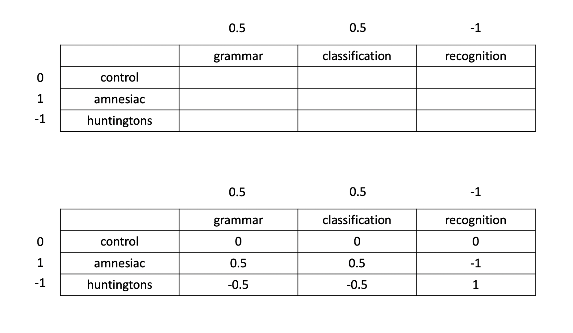
Specify the coefficients to be used in the contrast analysis, and present in a table.

Next, formally state the contrast that the researchers were interested in as testable hypotheses.

Hint

For an overview and example, review the manual contrasts flashcards.

We can specify the coefficients to be used in the contrast analysis in R using either:

Option 1

diag_coef  <- c('control' = 0, 'amnesic' = 1, 'huntingtons' = -1)
task_coef  <- c('grammar' = 0.5, 'classification' = 0.5, 'recognition' = -1)
contr_coef <- outer(diag_coef, task_coef)
contr_coef

            grammar classification recognition
control         0.0            0.0           0
amnesic         0.5            0.5          -1
huntingtons    -0.5           -0.5           1

Option 2

diag_coef  <- c('control' = 0, 'amnesic' = 1, 'huntingtons' = -1)
task_coef  <- c('grammar' = 0.5, 'classification' = 0.5, 'recognition' = -1)
contr_coef <- diag_coef %o% task_coef
contr_coef

            grammar classification recognition
control         0.0            0.0           0
amnesic         0.5            0.5          -1
huntingtons    -0.5           -0.5           1

Using either approach, we can then convert into a well-formatted table:

contr_coef %>% 
    kable(., caption = "Contrast Weights") %>%
    kable_styling(full_width = FALSE) 

Table 3: Contrast Weights

Contrast Weights

	grammar	classification	recognition
control	0.0	0.0	0
amnesic	0.5	0.5	-1
huntingtons	-0.5	-0.5	1

The above coefficients correspond to the following hypotheses:

\[ H_0: \quad \left(\frac{\mu_{2,1} + \mu_{2,2}}{2} - \mu_{2,3} \right) - \left( \frac{\mu_{3,1} + \mu_{3,2}}{2} - \mu_{3,3} \right) = 0 \]

\[ H_1: \quad \left(\frac{\mu_{2,1} + \mu_{2,2}}{2} - \mu_{2,3} \right) - \left( \frac{\mu_{3,1} + \mu_{3,2}}{2} - \mu_{3,3} \right) \neq 0 \]

which can be equivalently specified as:

\[ H_0: \quad \frac{\mu_{2,1} + \mu_{2,2}}{2} - \mu_{2,3} \quad = \quad \frac{\mu_{3,1} + \mu_{3,2}}{2} - \mu_{3,3} \]

\[ H_1: \quad \frac{\mu_{2,1} + \mu_{2,2}}{2} - \mu_{2,3} \quad \neq \quad \frac{\mu_{3,1} + \mu_{3,2}}{2} - \mu_{3,3} \]

both statements state that, in the population, the difference between the mean implicit memory and the explicit memory score is the same for individuals with amnesia and Huntingtons.

Note that the scores for the grammar and classification tasks have been averaged to obtain a single measure of ‘implicit memory’ score.

Question 6

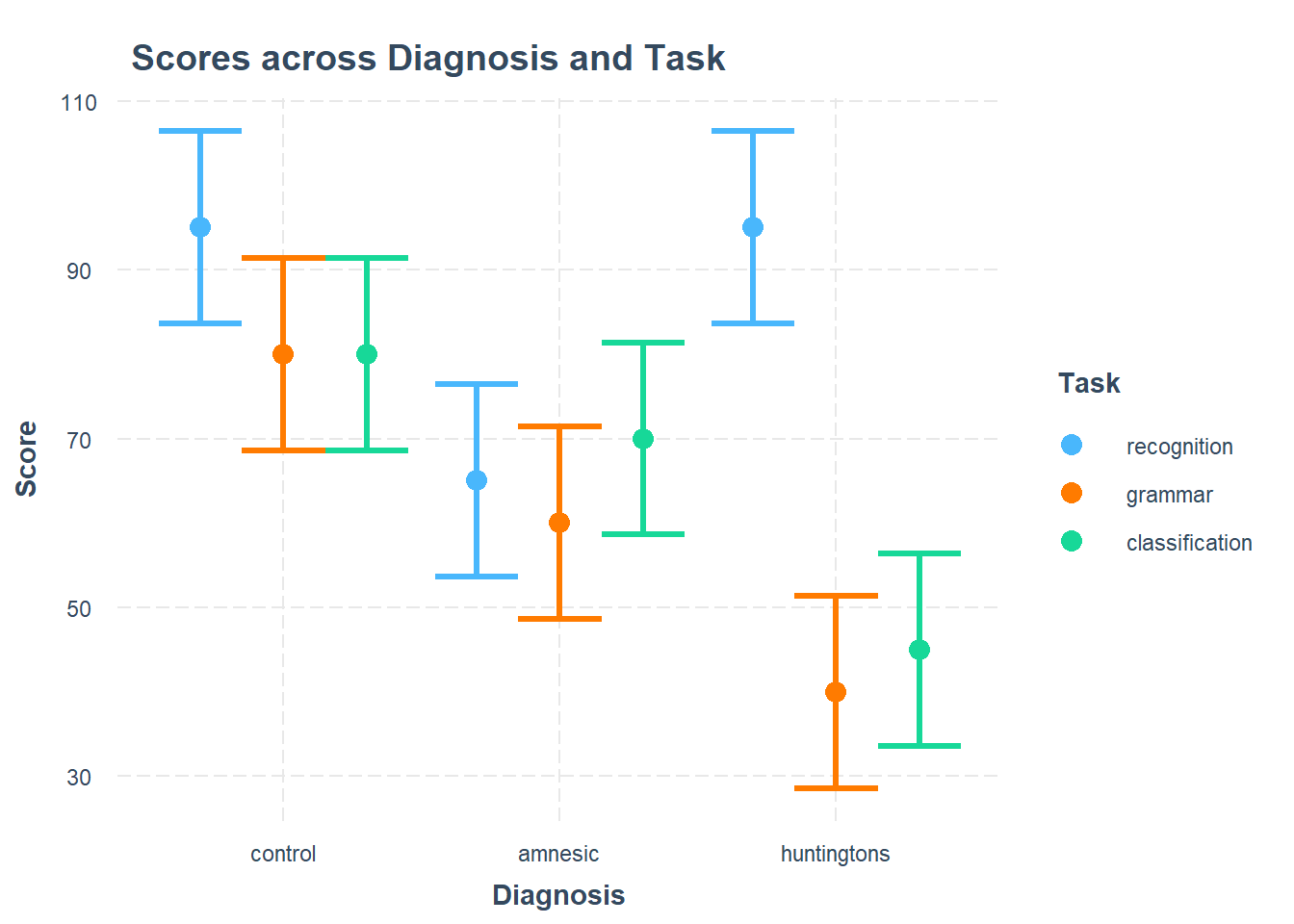
Firstly, use emmeans() to obtain the estimated means and uncertainties for your factors.

Next, specify the coefficients of the comparison and run the contrast analysis, obtaining 95% confidence intervals.

Report the results of the contrast analysis in full.

Hint

For an overview and example, review the manual contrasts flashcards.

Now that we have the coefficients, let’s firstly call the emmeans function to get the estimated means of our groups (this is also helpful to look at the ordering of the groups):

diag_task_mean <- emmeans(mdl_int, ~ Diagnosis*Task)
diag_task_mean

 Diagnosis   Task           emmean   SE df lower.CL upper.CL
 control     recognition        95 5.62 36     83.6    106.4
 amnesic     recognition        65 5.62 36     53.6     76.4
 huntingtons recognition        95 5.62 36     83.6    106.4
 control     grammar            80 5.62 36     68.6     91.4
 amnesic     grammar            60 5.62 36     48.6     71.4
 huntingtons grammar            40 5.62 36     28.6     51.4
 control     classification     80 5.62 36     68.6     91.4
 amnesic     classification     70 5.62 36     58.6     81.4
 huntingtons classification     45 5.62 36     33.6     56.4

Confidence level used: 0.95 

Next, from contr_coef, insert the coefficients following the order specified by the rows of diag_task_mean above. That is, the first one should be for control recognition and have a value of 0, the second for amnesic recognition with a value of -1, and so on…

Let’s specify our weights, and give a name to this contrast (in this example ‘Research Hyp’):

diag_task_comp <- contrast(diag_task_mean, 
                     method = list('Research Hyp' = c(0, -1, 1, 0, 0.5, -0.5, 0, 0.5, -0.5))
                     )

Next, let’s look at the output via one of two ways:

Option 1

#examine output
diag_task_comp

 contrast     estimate   SE df t.ratio p.value
 Research Hyp     52.5 9.73 36   5.396  <.0001

#obtain confidence intervals
confint(diag_task_comp)

 contrast     estimate   SE df lower.CL upper.CL
 Research Hyp     52.5 9.73 36     32.8     72.2

Confidence level used: 0.95 

Option 2

#examine summary output and state `infer = TRUE` to include confidence intervals
summary(diag_task_comp, infer = TRUE)

 contrast     estimate   SE df lower.CL upper.CL t.ratio p.value
 Research Hyp     52.5 9.73 36     32.8     72.2   5.396  <.0001

Confidence level used: 0.95 

We performed a test against \(H_0: \quad \frac{\mu_{2,1} + \mu_{2,2}}{2} - \mu_{2,3} \quad = \quad \frac{\mu_{3,1} + \mu_{3,2}}{2} - \mu_{3,3}\). At the 5% significance level, there was evidence that individuals with Amnesia and Huntingtons did differ in the difference between implicit and explicit memory tasks \((t(36) = 5.40, p < .001, \text{two-sided})\), and this difference was estimated to be 52.50. We are 95% confident that the difference in implicit and explicit memory scores between individuals with Amnesia and Huntingtons was between 32.80 to 72.20 points. Therefore, we can reject the null hypothesis that the difference in differences was equal to zero.

Simple Effects

Question 7

Examine the simple effects for Task at each level of Diagnosis; and then the simple effects for Diagnosis at each level of Task.

Hint

For an overview and example, review the simple effects flashcards.

Simple Effects of Task

From mdl_int_simple1 we can see the differences between tasks for each diagnosis group:

mdl_int_simple1 <- pairs(diag_task_mean, simple = "Task")
mdl_int_simple1

Diagnosis = control:
 contrast                     estimate   SE df t.ratio p.value
 recognition - grammar              15 7.94 36   1.888  0.1567
 recognition - classification       15 7.94 36   1.888  0.1567
 grammar - classification            0 7.94 36   0.000  1.0000

Diagnosis = amnesic:
 contrast                     estimate   SE df t.ratio p.value
 recognition - grammar               5 7.94 36   0.629  0.8050
 recognition - classification       -5 7.94 36  -0.629  0.8050
 grammar - classification          -10 7.94 36  -1.259  0.4273

Diagnosis = huntingtons:
 contrast                     estimate   SE df t.ratio p.value
 recognition - grammar              55 7.94 36   6.923  <.0001
 recognition - classification       50 7.94 36   6.294  <.0001
 grammar - classification           -5 7.94 36  -0.629  0.8050

P value adjustment: tukey method for comparing a family of 3 estimates 

Simple Effects of Diagnosis

From mdl_int_simple2 we can see the differences between diagnoses for each task group:

mdl_int_simple2 <- pairs(diag_task_mean, simple = "Diagnosis")
mdl_int_simple2

Task = recognition:
 contrast              estimate   SE df t.ratio p.value
 control - amnesic           30 7.94 36   3.776  0.0016
 control - huntingtons        0 7.94 36   0.000  1.0000
 amnesic - huntingtons      -30 7.94 36  -3.776  0.0016

Task = grammar:
 contrast              estimate   SE df t.ratio p.value
 control - amnesic           20 7.94 36   2.518  0.0424
 control - huntingtons       40 7.94 36   5.035  <.0001
 amnesic - huntingtons       20 7.94 36   2.518  0.0424

Task = classification:
 contrast              estimate   SE df t.ratio p.value
 control - amnesic           10 7.94 36   1.259  0.4273
 control - huntingtons       35 7.94 36   4.406  0.0003
 amnesic - huntingtons       25 7.94 36   3.147  0.0091

P value adjustment: tukey method for comparing a family of 3 estimates 

Question 8

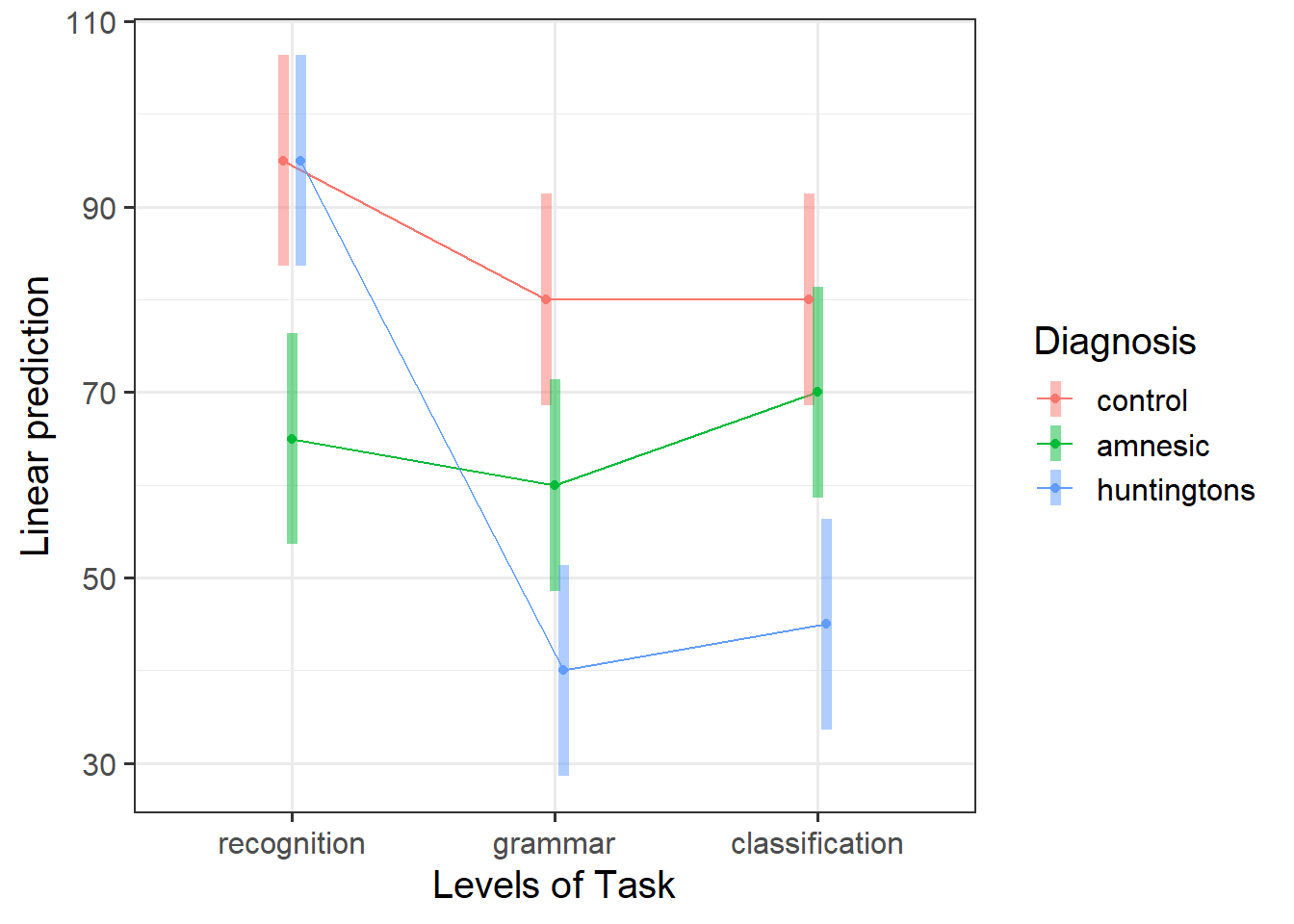
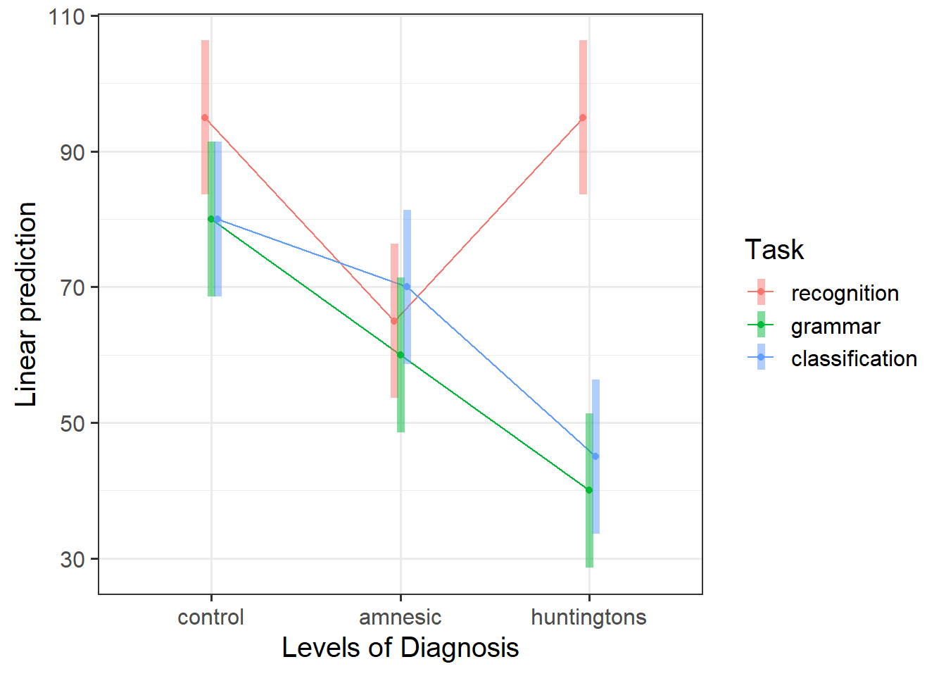
Visualise the interaction, displaying two plots - one with Diagnosis on the x-axis, and the other with Task on the x-axis.

Considering the simple effects that you noted above, identify the significant effects and match them to the corresponding points of your interaction plot.

Hint

For an overview and example, review the simple effects flashcards.

Recall that the patchwork package allows us to arrange multiple plots using either / or | or +.

Simple Effects of Task

plt_1 <- emmip(mdl_int, Diagnosis ~ Task, CIs = TRUE)
plt_1

For the simple effects of task (see plt_1), we saw the significant differences (those for which \(p<.05\)):

• Only in the Huntingtons group, between recognition & grammar and recognition & classification tasks
  • left-most blue point compared to the middle blue point, and then compared to the right-most blue point

Simple Effects of Diagnosis

plt_2 <- emmip(mdl_int, Task ~ Diagnosis, CIs = TRUE)
plt_2

For the simple effects of Diagnosis (see plt_2), we saw significant differences (those for which \(p<.05\)):

• in the recognition task, between control & amnesic
  • left-most red point to middle red point
• in the recognition task, between amnesic & huntingtons
  • middle red-point to right-most red point
• in the grammar task, between control & amnesic
  • left-most green point to middle green point
• in the grammar task, between control & huntingtons
  • left-most green point to right-most green point
• in the grammar task, between amnesic & huntingtons
  • middle green point to right-most green point
• in the classification task, between control & huntingtons
  • left-most blue point to right-most blue point
• in the classification task, between amnesic & huntingtons
  • middle blue point to right-most blue point

Pairwise Comparisons & Multiple Corrections

Question 9

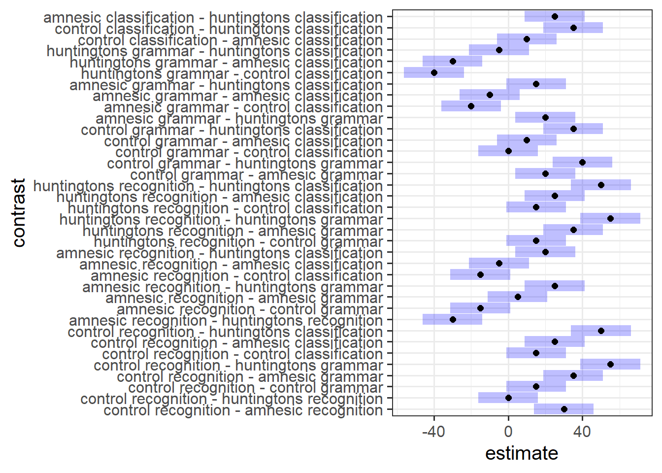
Conduct exploratory pairwise comparisons to compare all levels of Diagnosis with all levels of Task, applying no correction (note that Tukey will be automatically applied since we are comparing groups of means, so you will need to overwrite this).

Without adjusting our \(\alpha\) (or \(p\)-value), why might any inferences drawn from your output be problematic?

Hint

For an overview, review the multiple comparisons flashcards.

pairs_res <- pairs(diag_task_mean, adjust = "none")
pairs_res

 contrast                                             estimate   SE df t.ratio
 control recognition - amnesic recognition                  30 7.94 36   3.776
 control recognition - huntingtons recognition               0 7.94 36   0.000
 control recognition - control grammar                      15 7.94 36   1.888
 control recognition - amnesic grammar                      35 7.94 36   4.406
 control recognition - huntingtons grammar                  55 7.94 36   6.923
 control recognition - control classification               15 7.94 36   1.888
 control recognition - amnesic classification               25 7.94 36   3.147
 control recognition - huntingtons classification           50 7.94 36   6.294
 amnesic recognition - huntingtons recognition             -30 7.94 36  -3.776
 amnesic recognition - control grammar                     -15 7.94 36  -1.888
 amnesic recognition - amnesic grammar                       5 7.94 36   0.629
 amnesic recognition - huntingtons grammar                  25 7.94 36   3.147
 amnesic recognition - control classification              -15 7.94 36  -1.888
 amnesic recognition - amnesic classification               -5 7.94 36  -0.629
 amnesic recognition - huntingtons classification           20 7.94 36   2.518
 huntingtons recognition - control grammar                  15 7.94 36   1.888
 huntingtons recognition - amnesic grammar                  35 7.94 36   4.406
 huntingtons recognition - huntingtons grammar              55 7.94 36   6.923
 huntingtons recognition - control classification           15 7.94 36   1.888
 huntingtons recognition - amnesic classification           25 7.94 36   3.147
 huntingtons recognition - huntingtons classification       50 7.94 36   6.294
 control grammar - amnesic grammar                          20 7.94 36   2.518
 control grammar - huntingtons grammar                      40 7.94 36   5.035
 control grammar - control classification                    0 7.94 36   0.000
 control grammar - amnesic classification                   10 7.94 36   1.259
 control grammar - huntingtons classification               35 7.94 36   4.406
 amnesic grammar - huntingtons grammar                      20 7.94 36   2.518
 amnesic grammar - control classification                  -20 7.94 36  -2.518
 amnesic grammar - amnesic classification                  -10 7.94 36  -1.259
 amnesic grammar - huntingtons classification               15 7.94 36   1.888
 huntingtons grammar - control classification              -40 7.94 36  -5.035
 huntingtons grammar - amnesic classification              -30 7.94 36  -3.776
 huntingtons grammar - huntingtons classification           -5 7.94 36  -0.629
 control classification - amnesic classification            10 7.94 36   1.259
 control classification - huntingtons classification        35 7.94 36   4.406
 amnesic classification - huntingtons classification        25 7.94 36   3.147
 p.value
  0.0006
  1.0000
  0.0671
  0.0001
  <.0001
  0.0671
  0.0033
  <.0001
  0.0006
  0.0671
  0.5331
  0.0033
  0.0671
  0.5331
  0.0164
  0.0671
  0.0001
  <.0001
  0.0671
  0.0033
  <.0001
  0.0164
  <.0001
  1.0000
  0.2162
  0.0001
  0.0164
  0.0164
  0.2162
  0.0671
  <.0001
  0.0006
  0.5331
  0.2162
  0.0001
  0.0033

#can also plot if you'd like:
plot(pairs_res)

From the above, we can see comparisons for all different possible pairs of diagnosis-task combinations¹.

In total, there are 9 different estimates, but comparing them all means that we have 36 comparisons being tested! By not adjusting our \(p\)-value, we are increasing the experiment-wise Type I error rate - we could wrongly reject the null hypothesis at a much higher rate than 5/100 (or 1/20 as is assumed when \(\alpha = .05\)). To overcome this, we might adjust and determine a result to be statistically significant if \(p < .005\), as opposed to \(p < .05\), depending on how many tests are in our family of tests.

Question 10

Select an appropriate method to adjust for multiple comparisons, and then obtain confidence intervals.

Comment on how these \(p\)-values differ from your raw (i.e., unadjusted) \(p\)-values.

Hint

For an overview, review the multiple comparisons flashcards.

Note what the functions in R do is adjust the \(p\)-value, rather than the \(\alpha\).

Since we’re interested in all pairwise comparisons of means, the Tukey adjustment might be a sensible approach. However, we’ll also show the Bonferroni to show how it differs (note, in practice you would only apply one correction and justify this choice based on your design - we are only applying two to note how they differ!)

Tukey

contrast(diag_task_mean, method = "pairwise", adjust="Tukey")

 contrast                                             estimate   SE df t.ratio
 control recognition - amnesic recognition                  30 7.94 36   3.776
 control recognition - huntingtons recognition               0 7.94 36   0.000
 control recognition - control grammar                      15 7.94 36   1.888
 control recognition - amnesic grammar                      35 7.94 36   4.406
 control recognition - huntingtons grammar                  55 7.94 36   6.923
 control recognition - control classification               15 7.94 36   1.888
 control recognition - amnesic classification               25 7.94 36   3.147
 control recognition - huntingtons classification           50 7.94 36   6.294
 amnesic recognition - huntingtons recognition             -30 7.94 36  -3.776
 amnesic recognition - control grammar                     -15 7.94 36  -1.888
 amnesic recognition - amnesic grammar                       5 7.94 36   0.629
 amnesic recognition - huntingtons grammar                  25 7.94 36   3.147
 amnesic recognition - control classification              -15 7.94 36  -1.888
 amnesic recognition - amnesic classification               -5 7.94 36  -0.629
 amnesic recognition - huntingtons classification           20 7.94 36   2.518
 huntingtons recognition - control grammar                  15 7.94 36   1.888
 huntingtons recognition - amnesic grammar                  35 7.94 36   4.406
 huntingtons recognition - huntingtons grammar              55 7.94 36   6.923
 huntingtons recognition - control classification           15 7.94 36   1.888
 huntingtons recognition - amnesic classification           25 7.94 36   3.147
 huntingtons recognition - huntingtons classification       50 7.94 36   6.294
 control grammar - amnesic grammar                          20 7.94 36   2.518
 control grammar - huntingtons grammar                      40 7.94 36   5.035
 control grammar - control classification                    0 7.94 36   0.000
 control grammar - amnesic classification                   10 7.94 36   1.259
 control grammar - huntingtons classification               35 7.94 36   4.406
 amnesic grammar - huntingtons grammar                      20 7.94 36   2.518
 amnesic grammar - control classification                  -20 7.94 36  -2.518
 amnesic grammar - amnesic classification                  -10 7.94 36  -1.259
 amnesic grammar - huntingtons classification               15 7.94 36   1.888
 huntingtons grammar - control classification              -40 7.94 36  -5.035
 huntingtons grammar - amnesic classification              -30 7.94 36  -3.776
 huntingtons grammar - huntingtons classification           -5 7.94 36  -0.629
 control classification - amnesic classification            10 7.94 36   1.259
 control classification - huntingtons classification        35 7.94 36   4.406
 amnesic classification - huntingtons classification        25 7.94 36   3.147
 p.value
  0.0149
  1.0000
  0.6257
  0.0026
  <.0001
  0.6257
  0.0711
  <.0001
  0.0149
  0.6257
  0.9993
  0.0711
  0.6257
  0.9993
  0.2575
  0.6257
  0.0026
  <.0001
  0.6257
  0.0711
  <.0001
  0.2575
  0.0004
  1.0000
  0.9367
  0.0026
  0.2575
  0.2575
  0.9367
  0.6257
  0.0004
  0.0149
  0.9993
  0.9367
  0.0026
  0.0711

P value adjustment: tukey method for comparing a family of 9 estimates 

Note that 8 of the comparisons are no longer significant when using Tukey’s adjustment, suggesting that these might have been (when using no adjustment) Type I errors!

Bonferroni

contrast(diag_task_mean, method = "pairwise", adjust="bonferroni")

 contrast                                             estimate   SE df t.ratio
 control recognition - amnesic recognition                  30 7.94 36   3.776
 control recognition - huntingtons recognition               0 7.94 36   0.000
 control recognition - control grammar                      15 7.94 36   1.888
 control recognition - amnesic grammar                      35 7.94 36   4.406
 control recognition - huntingtons grammar                  55 7.94 36   6.923
 control recognition - control classification               15 7.94 36   1.888
 control recognition - amnesic classification               25 7.94 36   3.147
 control recognition - huntingtons classification           50 7.94 36   6.294
 amnesic recognition - huntingtons recognition             -30 7.94 36  -3.776
 amnesic recognition - control grammar                     -15 7.94 36  -1.888
 amnesic recognition - amnesic grammar                       5 7.94 36   0.629
 amnesic recognition - huntingtons grammar                  25 7.94 36   3.147
 amnesic recognition - control classification              -15 7.94 36  -1.888
 amnesic recognition - amnesic classification               -5 7.94 36  -0.629
 amnesic recognition - huntingtons classification           20 7.94 36   2.518
 huntingtons recognition - control grammar                  15 7.94 36   1.888
 huntingtons recognition - amnesic grammar                  35 7.94 36   4.406
 huntingtons recognition - huntingtons grammar              55 7.94 36   6.923
 huntingtons recognition - control classification           15 7.94 36   1.888
 huntingtons recognition - amnesic classification           25 7.94 36   3.147
 huntingtons recognition - huntingtons classification       50 7.94 36   6.294
 control grammar - amnesic grammar                          20 7.94 36   2.518
 control grammar - huntingtons grammar                      40 7.94 36   5.035
 control grammar - control classification                    0 7.94 36   0.000
 control grammar - amnesic classification                   10 7.94 36   1.259
 control grammar - huntingtons classification               35 7.94 36   4.406
 amnesic grammar - huntingtons grammar                      20 7.94 36   2.518
 amnesic grammar - control classification                  -20 7.94 36  -2.518
 amnesic grammar - amnesic classification                  -10 7.94 36  -1.259
 amnesic grammar - huntingtons classification               15 7.94 36   1.888
 huntingtons grammar - control classification              -40 7.94 36  -5.035
 huntingtons grammar - amnesic classification              -30 7.94 36  -3.776
 huntingtons grammar - huntingtons classification           -5 7.94 36  -0.629
 control classification - amnesic classification            10 7.94 36   1.259
 control classification - huntingtons classification        35 7.94 36   4.406
 amnesic classification - huntingtons classification        25 7.94 36   3.147
 p.value
  0.0207
  1.0000
  1.0000
  0.0033
  <.0001
  1.0000
  0.1190
  <.0001
  0.0207
  1.0000
  1.0000
  0.1190
  1.0000
  1.0000
  0.5907
  1.0000
  0.0033
  <.0001
  1.0000
  0.1190
  <.0001
  0.5907
  0.0005
  1.0000
  1.0000
  0.0033
  0.5907
  0.5907
  1.0000
  1.0000
  0.0005
  0.0207
  1.0000
  1.0000
  0.0033
  0.1190

P value adjustment: bonferroni method for 36 tests 

The first Bonferroni adjusted \(p\)-value is 0.0207.

The raw (unadjusted) \(p\)-value from the previous question was 0.0005759265.

The Bonferroni method simply multiplies the ‘raw’ \(p\)-value by the number of the tests, which we know is 36.

0.0005759265 * 36

[1] 0.02073335

In terms of differences in Bonferroni to raw \(p\)-values, they are thus 36 times the size.

One benefit of Bonferroni is that it can be applied to any set of \(p\)-values, whereas Tukey only applies when comparing the means of levels of a factor. The downside, however, is that it may be overly conservative (i.e. reduce our power to detect an effect that is truly there).

Compile Report

Compile Report

Knit your report to PDF, and check over your work. To do so, you should make sure:

• Only the output you want your reader to see is visible (e.g., do you want to hide your code?)
• Check that the tinytex package is installed
• Ensure that the ‘yaml’ (bit at the very top of your document) looks something like this:

---
title: "this is my report title"
author: "B1234506"
date: "07/09/2024"
output: bookdown::pdf_document2
---

What to do if you cannot knit to PDF

If you are having issues knitting directly to PDF, try the following:

• Knit to HTML file
  
• Open your HTML in a web-browser (e.g. Chrome, Firefox)
  
• Print to PDF (Ctrl+P, then choose to save to PDF)
  
• Open file to check formatting

Hiding Code and/or Output

Hiding R Code

To not show the code of an R code chunk, and only show the output, write:

```{r, echo=FALSE}
# code goes here
```

Hiding R Output

To show the code of an R code chunk, but hide the output, write:

```{r, results='hide'}
# code goes here
```

Hiding R Code and Output

To hide both code and output of an R code chunk, write:

```{r, include=FALSE}
# code goes here
```

Tinytex

You must make sure you have tinytex installed in R so that you can “Knit” your Rmd document to a PDF file:

install.packages("tinytex")
tinytex::install_tinytex()

You should end up with a PDF file. If you have followed the above instructions and still have issues with knitting, speak with a Tutor.

Footnotes

1. the differences between the group means for the comparison as labelled