Model Fit and Comparisons

Learning Objectives

At the end of this lab, you will:

1. Understand how to calculate the interpret \(R^2\) and adjusted-\(R^2\) as a measure of model quality.
2. Understand the calculation and interpretation of the \(F\)-test of model utility.
3. Understand measures of model fit using \(F\).
   
4. Understand the principles of model selection and how to compare models via \(F\) tests, \(AIC\), and \(BIC\).

What You Need

1. Be up to date with lectures
2. Have completed Week 1 and Week 2, and Week 3 lab exercises

Required R Packages

Remember to load all packages within a code chunk at the start of your RMarkdown file using library(). If you do not have a package and need to install, do so within the console using install.packages(" "). For further guidance on installing/updating packages, see Section C here.

For this lab, you will need to load the following package(s):

• tidyverse
• sjPlot
• kableExtra

Presenting Results

All results should be presented following APA guidelines.If you need a reminder on how to hide code, format tables/plots, etc., make sure to review the rmd bootcamp.

The example write-up sections included as part of the solutions are not perfect - they instead should give you a good example of what information you should include and how to structure this. Note that you must not copy any of the write-ups included below for future reports - if you do, you will be committing plagiarism, and this type of academic misconduct is taken very seriously by the University. You can find out more here.

Lab Data

You can download the data required for this lab here or read it in via this link https://uoepsy.github.io/data/wellbeing_rural.csv

Study Overview

Research Question(s)

Section I

• Is there an association between wellbeing and time spent outdoors after taking into account the association between wellbeing and social interactions?

Section II

• RQ1: Is the number of weekly social interactions a useful predictor of wellbeing scores?
• RQ2: Does weekly outdoor time explain a significant amount of variance in wellbeing scores over and above social interactions?

Wellbeing/Rurality data codebook.

Description

From the Edinburgh & Lothians, 100 city/suburb residences and 100 rural residences were chosen at random and contacted to participate in the study. The Warwick-Edinburgh Mental Wellbeing Scale (WEMWBS) was used to measure mental health and well-being.

Participants filled out a questionnaire including items concerning: estimated average number of hours spent outdoors each week, estimated average number of social interactions each week (whether on-line or in-person), whether a daily routine is followed (yes/no). For those respondents who had an activity tracker app or smart watch, they were asked to provide their average weekly number of steps.

Data Dictionary

The data in wellbeing_rural.csv contain seven attributes collected from a random sample of \(n=200\) hypothetical residents over Edinburgh & Lothians, and include:

variable	description
age	Age in years of respondent
outdoor_time	Self report estimated number of hours per week spent outdoors
social_int	Self report estimated number of social interactions per week (both online and in-person)
routine	Binary 1=Yes/0=No response to the question 'Do you follow a daily routine throughout the week?'
wellbeing	Warwick-Edinburgh Mental Wellbeing Scale (WEMWBS), a self-report measure of mental health and well-being. The scale is scored by summing responses to each item, with items answered on a 1 to 5 Likert scale. The minimum scale score is 14 and the maximum is 70
location	Location of primary residence (City, Suburb, Rural)
steps_k	Average weekly number of steps in thousands (as given by activity tracker if available)

Preview

The first six rows of the data are:

age	outdoor_time	social_int	routine	wellbeing	location	steps_k
28	12	13	1	36	rural	21.6
56	5	15	1	41	rural	12.3
25	19	11	1	35	rural	49.8
60	25	15	0	35	rural	NA
19	9	18	1	32	rural	48.1
34	18	13	1	34	rural	67.3

Setup

Setup

1. Create a new RMarkdown file
2. Load the required package(s)
3. Read the wellbeing dataset into R, assigning it to an object named mwdata

#Loading the required package(s)
library(tidyverse)
library(sjPlot)
library(kableExtra)

# Reading in data and storing to an object named 'mwdata'
mwdata <- read_csv("https://uoepsy.github.io/data/wellbeing_rural.csv")

Exercises

Section I: Model Fit

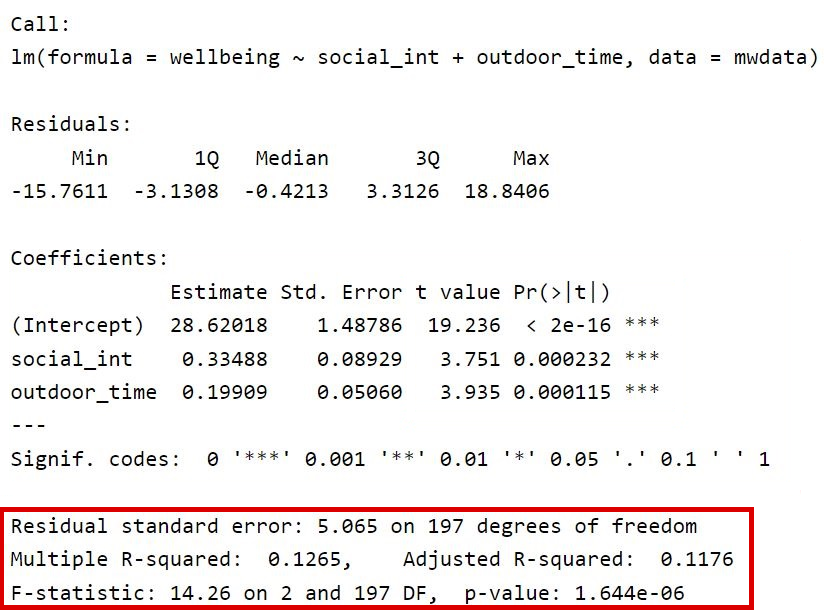
In the first section of this lab, you will focus on the statistics contained within the highlighted sections of the summary() output below. You will be both calculating these by hand and deriving via R before interpreting these values in the context of the research question.

Question 1

Fit the following multiple linear regression model, and assign the output to an object called mdl.

\[ \text{Wellbeing} = \beta_0 + \beta_1 \cdot Social~Interactions + \beta_2 \cdot Outdoor~Time + \epsilon \]

Hint

This is the same model that you have fitted in the previous couple of weeks.

We can fit our multiple regression model using the lm() function.

For a recap, see the statistical models flashcards, specifically the multiple linear regression models - description & specification card.

mdl <- lm(wellbeing ~ social_int + outdoor_time, data = mwdata)
summary(mdl)

Call:
lm(formula = wellbeing ~ social_int + outdoor_time, data = mwdata)

Residuals:
     Min       1Q   Median       3Q      Max 
-15.7611  -3.1308  -0.4213   3.3126  18.8406 

Coefficients:
             Estimate Std. Error t value Pr(>|t|)    
(Intercept)  28.62018    1.48786  19.236  < 2e-16 ***
social_int    0.33488    0.08929   3.751 0.000232 ***
outdoor_time  0.19909    0.05060   3.935 0.000115 ***
---
Signif. codes:  0 '***' 0.001 '**' 0.01 '*' 0.05 '.' 0.1 ' ' 1

Residual standard error: 5.065 on 197 degrees of freedom
Multiple R-squared:  0.1265,    Adjusted R-squared:  0.1176 
F-statistic: 14.26 on 2 and 197 DF,  p-value: 1.644e-06

Question 2

What is the proportion of the total variability in wellbeing scores explained by the model?

Hint

The proportion of the total variability explained is given by \(R^2\). Since the model includes 2 predictors, you should report the Adjusted-\(R^2\).

For a more detailed overview, see the R-squared and Adjusted R-squared flashcard.

Manually

In R we can write:

#Define n & k
n <- nrow(mwdata)
k <- 2

#Predicted scores
wellbeing_fitted <- mwdata %>%
  mutate(
    wellbeing_pred = predict(mdl),
    wellbeing_resid = wellbeing - wellbeing_pred)

# Sums of Squares, and R / Adjusted R Squared
wellbeing_fitted %>%
  summarise(
    SSModel = sum((wellbeing_pred - mean(wellbeing))^2),
    SSTotal = sum((wellbeing - mean(wellbeing))^2),
    SSResid = sum(wellbeing_resid^2)
  ) %>% 
  summarise(
    RSquared = SSModel / SSTotal,
    AdjRSquared = 1-((1-(RSquared))*(n-1)/(n-k-1))
  )

# A tibble: 1 × 2
  RSquared AdjRSquared
     <dbl>       <dbl>
1    0.126       0.118

The output displays the Adjusted \(R^2\) value in the following column:

AdjRSquared
 <dbl>
 0.118

R Function

#look in second bottom row - Multiple R Squared and Adjusted R Squared both reported here
summary(mdl)

Call:
lm(formula = wellbeing ~ social_int + outdoor_time, data = mwdata)

Residuals:
     Min       1Q   Median       3Q      Max 
-15.7611  -3.1308  -0.4213   3.3126  18.8406 

Coefficients:
             Estimate Std. Error t value Pr(>|t|)    
(Intercept)  28.62018    1.48786  19.236  < 2e-16 ***
social_int    0.33488    0.08929   3.751 0.000232 ***
outdoor_time  0.19909    0.05060   3.935 0.000115 ***
---
Signif. codes:  0 '***' 0.001 '**' 0.01 '*' 0.05 '.' 0.1 ' ' 1

Residual standard error: 5.065 on 197 degrees of freedom
Multiple R-squared:  0.1265,    Adjusted R-squared:  0.1176 
F-statistic: 14.26 on 2 and 197 DF,  p-value: 1.644e-06

The output of summary() displays the Adjusted \(R^2\) value in the following line:

Adjusted R-squared:  0.1176 

Approximately 12% of the total variability in wellbeing scores is accounted for by social interactions and outdoor time.

Question 3

What do you notice about the unadjusted and adjusted \(R^2\) values?

Hint

Are they similar or quite different? Why might this be?

Think about when you would report \(R^2\) and Adjusted-\(R^2\) - the R-squared and Adjusted R-squared flashcard has some detail on this, but it will also be useful to think about how each is calculated.

The values of the unadjusted (0.1265) and adjusted \(R^2\) (0.1176) values are quite similar. This is because the sample size is quite large \((n = 200)\), and the number of predictors \((k = 2)\) is small.

Question 4

Perform a model utility test at the 5% significance level and report your results.

In other words, conduct an \(F\)-test against the null hypothesis that the model is ineffective at predicting wellbeing scores using social interactions and outdoor time by computing the \(F\)-statistic using its definition.

Hint

The \(F\)-ratio is used to test the null hypothesis that all regression slopes are zero.

See the F-ratio flashcard for a more detailed overview.

Manually

#df(model) = k 
df1 <- 2

#df(residual) = n - k - 1
df2 <- nrow(mwdata) - 2 - 1

f_star <- qf(0.95, df1, df2)

#check value
f_star

[1] 3.041753

model_utility <- wellbeing_fitted %>%
  summarise(
    SSModel = sum((wellbeing_pred - mean(wellbeing))^2),
    SSResid = sum(wellbeing_resid^2),
    MSModel = SSModel / df1,
    MSResid = SSResid / df2,
    FObs = MSModel / MSResid
  )
model_utility

# A tibble: 1 × 5
  SSModel SSResid MSModel MSResid  FObs
    <dbl>   <dbl>   <dbl>   <dbl> <dbl>
1    732.   5054.    366.    25.7  14.3

We can also compute the p-value:

pvalue <- 1 - pf(model_utility$FObs, df1, df2)
pvalue

[1] 1.643779e-06

The value 1.643779e-06 simply means \(1.6 \times 10^{-6}\), so it’s a really small number (i.e., 0.000001643779).

R Function

#look in bottom row
summary(mdl)

Call:
lm(formula = wellbeing ~ social_int + outdoor_time, data = mwdata)

Residuals:
     Min       1Q   Median       3Q      Max 
-15.7611  -3.1308  -0.4213   3.3126  18.8406 

Coefficients:
             Estimate Std. Error t value Pr(>|t|)    
(Intercept)  28.62018    1.48786  19.236  < 2e-16 ***
social_int    0.33488    0.08929   3.751 0.000232 ***
outdoor_time  0.19909    0.05060   3.935 0.000115 ***
---
Signif. codes:  0 '***' 0.001 '**' 0.01 '*' 0.05 '.' 0.1 ' ' 1

Residual standard error: 5.065 on 197 degrees of freedom
Multiple R-squared:  0.1265,    Adjusted R-squared:  0.1176 
F-statistic: 14.26 on 2 and 197 DF,  p-value: 1.644e-06

The relevant row is the following:

F-statistic: 14.26 on 2 and 197 DF,  p-value: 1.644e-06

We performed an \(F\)-test of model utility at the 5% significance level, where \(F(2,197) = 14.26, p <.001\).

The large \(F\)-statistic and small \(p\)-value \((p <.001)\) suggested that we have very strong evidence against the null hypothesis.

In other words, the data provide strong evidence that the number of social interactions and outdoor time are predictors of wellbeing scores.

Section II: Model Comparisons

In the second section of this lab, you will focus on model comparison where you will formally test a number of research questions:

• RQ1: Is the number of weekly social interactions a useful predictor of wellbeing scores?
• RQ2: Does weekly outdoor time explain a significant amount of variance in wellbeing scores over and above the number of weekly social interactions?

Question 5

Fit the below 3 models required to address the 2 research questions stated above. Note down which model(s) will be used to address each research question, and examine the results of each model.

Name the models as follows: “wb_mdl0”, “wb_mdl1”, “wb_mdl2”

\[ \text{Wellbeing} = \beta_0 + \epsilon \]

\[ \text{Wellbeing} = \beta_0 + \beta_1 \cdot Social~Interactions + \epsilon \]

\[ \text{Wellbeing} = \beta_0 + \beta_1 \cdot Social~Interactions + \beta_2 \cdot Outdoor~Time + \epsilon \]

Hint

We can fit our multiple regression models individually using the lm() function. For a recap, see the statistical models flashcards, specifically the multiple linear regression models - description & specification card.

The summary() function will be useful to examine the model output.

wb_mdl0

#null/intercept only model
wb_mdl0 <- lm(wellbeing ~ 1, data = mwdata)
summary(wb_mdl0)

Call:
lm(formula = wellbeing ~ 1, data = mwdata)

Residuals:
    Min      1Q  Median      3Q     Max 
-14.295  -3.295  -1.295   3.705  22.705 

Coefficients:
            Estimate Std. Error t value Pr(>|t|)    
(Intercept)  36.2950     0.3813   95.19   <2e-16 ***
---
Signif. codes:  0 '***' 0.001 '**' 0.01 '*' 0.05 '.' 0.1 ' ' 1

Residual standard error: 5.392 on 199 degrees of freedom

wb_mdl1

#model with social interactions
wb_mdl1 <- lm(wellbeing ~ social_int, data = mwdata)
summary(wb_mdl1)

Call:
lm(formula = wellbeing ~ social_int, data = mwdata)

Residuals:
     Min       1Q   Median       3Q      Max 
-15.5628  -3.2741  -0.7908   3.3703  20.4706 

Coefficients:
            Estimate Std. Error t value Pr(>|t|)    
(Intercept) 32.40771    1.17532  27.573  < 2e-16 ***
social_int   0.32220    0.09243   3.486 0.000605 ***
---
Signif. codes:  0 '***' 0.001 '**' 0.01 '*' 0.05 '.' 0.1 ' ' 1

Residual standard error: 5.247 on 198 degrees of freedom
Multiple R-squared:  0.05781,   Adjusted R-squared:  0.05306 
F-statistic: 12.15 on 1 and 198 DF,  p-value: 0.0006045

wb_mdl2

#model with social interactions and outdoor time
wb_mdl2 <- lm(wellbeing ~ social_int + outdoor_time, data = mwdata)
summary(wb_mdl2)

Call:
lm(formula = wellbeing ~ social_int + outdoor_time, data = mwdata)

Residuals:
     Min       1Q   Median       3Q      Max 
-15.7611  -3.1308  -0.4213   3.3126  18.8406 

Coefficients:
             Estimate Std. Error t value Pr(>|t|)    
(Intercept)  28.62018    1.48786  19.236  < 2e-16 ***
social_int    0.33488    0.08929   3.751 0.000232 ***
outdoor_time  0.19909    0.05060   3.935 0.000115 ***
---
Signif. codes:  0 '***' 0.001 '**' 0.01 '*' 0.05 '.' 0.1 ' ' 1

Residual standard error: 5.065 on 197 degrees of freedom
Multiple R-squared:  0.1265,    Adjusted R-squared:  0.1176 
F-statistic: 14.26 on 2 and 197 DF,  p-value: 1.644e-06

The models required to address each research question (RQ) are:

• RQ1: Models wb_mdl0 and wb_mdl1
• RQ2: Models wb_mdl1 and wb_mdl2

Question 6

RQ1: Is the number of weekly social interactions a useful predictor of wellbeing scores?

Check that the \(F\)-statistic and the \(p\)-value are the same from the model comparison as that which are given at the bottom of summary(wb_mdl1).

Provide the key model results from the two models in a single formatted table.

Hint

Remember that the null model tests the null hypothesis that all beta coefficients are zero. By comparing wb_mdl0 to wb_mdl1, we can test whether we should include the IV of ‘social_int’.

When considering what method(s) you can use to compare the models, remember to determine whether the models are nested or non-nested.

You can use KableExtra to present your model comparison results in a well formatted table. For a quick guide, review the tables flashcard.

Model Comparison

Run model comparison via anova(), and present results in well formatted table:

anova(wb_mdl0, wb_mdl1) %>%
    kable(caption = "Model Comparison - wb_mdl0 vs wb_mdl1", align = "c", digits = c(2,2,2,2,2,4)) %>%
    kable_styling(full_width = FALSE)

Table 1: Model Comparison - wb_mdl0 vs wb_mdl1

Model Comparison - wb_mdl0 vs wb_mdl1

Res.Df	RSS	Df	Sum of Sq	F	Pr(>F)
199	5785.6	NA	NA	NA	NA
198	5451.1	1	334.49	12.15	6e-04

Comparing summary() and anova() Outputs

The output of anova(wb_mdl0, wb_mdl1) displays the \(F\)-statistic and the \(p\)-value in the following line:

  Res.Df    RSS Df Sum of Sq     F    Pr(>F)  
2    198 5451.1  1    334.49 12.15 0.0006045 ***

We can check that the \(F\)-statistic and the \(p\)-value are the the same as that which is given at the bottom of summary(wb_mdl1):

F-statistic: 12.15 on 1 and 198 DF,  p-value: 0.0006045

The \(F\)-statistic and the \(p\)-value from anova(wb_mdl0, wb_mdl1) and summary(wb_mdl1) both match! This is because the \(F\)-test from a model with a single predictor (i.e, ‘wb_mdl1’) is really just a comparison against the null model (i.e, ‘wb_mdl0’).

Table of Model Results

tab_model(wb_mdl0, wb_mdl1,
          dv.labels = c("Wellbeing (WEMWBS Scores)", "Wellbeing (WEMWBS Scores)"),
          pred.labels = c("social_int" = "Social Interactions (number per week)"),
          title = "Regression Table for Wellbeing Models wb0 and wb1")

Table 2: Regression Table for Wellbeing Models wb0 and wb1

Regression Table for Wellbeing Models wb0 and wb1

	Wellbeing (WEMWBS Scores)			Wellbeing (WEMWBS Scores)
Predictors	Estimates	CI	p	Estimates	CI	p
(Intercept)	36.29	35.54 – 37.05	<0.001	32.41	30.09 – 34.73	<0.001
Social Interactions (number per week)				0.32	0.14 – 0.50	0.001
Observations	200			200
R2 / R2 adjusted	0.000 / 0.000			0.058 / 0.053

The number of social interactions was found to explain a significant amount of variance in wellbeing scores \((F(1 ,198) = 12.15, p<.001)\). The model with social interactions was significantly better fitting than the intercept-only model, and thus social interactions is a useful predictor of wellbeing scores. Full regression results are presented in Table 2.

Question 7

Look at the amount of variation in wellbeing scores explained by models “wb_mdl1” and “wb_mdl2”.

From this, can we answer the second research question of whether weekly outdoor time explains a significant amount of variance in wellbeing scores over and above social interactions?

Provide justification/rationale for your answer.

Hint

You will need to review the \(R^2\) and Adjusted \(R^2\) values.

Consider whether comparing these numeric values would constitute a statistical comparison.

Let’s look at the amount of variance explained by each model:

summary(wb_mdl1)$r.squared

[1] 0.0578147

summary(wb_mdl2)$adj.r.squared

[1] 0.1176021

The model with weekly outdoor time as a predictor explains 12% of the variance, and the model without explains 6%. But, from only looking at the proportion of variance accounted for in each model, we cannot determine which model is statistically a better fit.

To answer the question ‘Does including weekly outdoor time as a predictor provide a significantly better fit of the data?’ we need to statistically compare wb_mdl1 to wb_mdl2.

Question 8

Does weekly outdoor time explain a significant amount of variance in wellbeing scores over and above social interactions?

Hint

To address RQ2, you need to statistically compare “wb_mdl1” and “wb_mdl2”.

When considering what method(s) you can use to compare the models, remember to determine whether the models are nested or non-nested.

You can use KableExtra to present your model comparison results in a well formatted table. For a quick guide, review the tables flashcard.

Model Comparison

To statistically compare models, we could use an incremental \(F\)-test to compare the models since the models are nested and from the same dataset:

anova(wb_mdl1, wb_mdl2) %>%
    kable(caption = "Model Comparison - wb_mdl1 vs wb_mdl2", align = "c", digits = c(2,2,2,2,2,4)) %>%
    kable_styling(full_width = FALSE)

Table 3: Model Comparison - wb_mdl1 vs wb_mdl2

Model Comparison - wb_mdl1 vs wb_mdl2

Res.Df	RSS	Df	Sum of Sq	F	Pr(>F)
198	5451.10	NA	NA	NA	NA
197	5053.89	1	397.21	15.48	1e-04

Table of Model Results

Present results from both models:

tab_model(wb_mdl1, wb_mdl2,
          dv.labels = c("Wellbeing (WEMWBS Scores)", "Wellbeing (WEMWBS Scores)"),
          pred.labels = c("social_int" = "Social Interactions (number per week)",
                          "outdoor_time" = "Outdoor Time (hours per week)"),
          title = "Regression Table for Wellbeing Models wb1 and wb2")

Table 4: Regression Table for Wellbeing Models wb1 and wb2

Regression Table for Wellbeing Models wb1 and wb2

	Wellbeing (WEMWBS Scores)			Wellbeing (WEMWBS Scores)
Predictors	Estimates	CI	p	Estimates	CI	p
(Intercept)	32.41	30.09 – 34.73	<0.001	28.62	25.69 – 31.55	<0.001
Social Interactions (number per week)	0.32	0.14 – 0.50	0.001	0.33	0.16 – 0.51	<0.001
Outdoor Time (hours per week)				0.20	0.10 – 0.30	<0.001
Observations	200			200
R2 / R2 adjusted	0.058 / 0.053			0.126 / 0.118

As presented in Table 3, weekly outdoor time was found to explain a significant amount of variance in wellbeing scores over and above weekly social interactions \((F(1 ,197) = 15.48, p<.001)\).

Question 9

A fellow researcher has suggested to examine the role of age in wellbeing scores. Based on their recommendation, compare the two following models, each looking at the associations of Wellbeing scores and different predictor variables.

\(\text{Wellbeing} = \beta_0 + \beta_1 \cdot \text{Social~Interactions} + \beta_2 \cdot \text{Age} + \epsilon\)

\(\text{Wellbeing} = \beta_0 + \beta_1 \cdot \text{Outdoor~Time} + \epsilon\)

Report which model you think best fits the data, and justify your answer.

Hint

Are the models are nested or non-nested? This will impact what method(s) you can use to compare the models.

Solution

Solution 1.

#fit models
wb_socint_age <- lm(wellbeing ~ social_int + age, data = mwdata)
wb_outdoor <- lm(wellbeing ~ outdoor_time, data = mwdata)

#AIC values
AIC(wb_socint_age, wb_outdoor)

              df      AIC
wb_socint_age  4 1236.575
wb_outdoor     3 1233.289

#BIC values
BIC(wb_socint_age, wb_outdoor)

              df      BIC
wb_socint_age  4 1249.769
wb_outdoor     3 1243.184

We used \(AIC\) and \(BIC\) model selection to distinguish between two possible models describing the association between several personal factors and wellbeing scores. The model with outdoor time included as a single predictor was better fitting \((AIC = 1233.29)\) than the alternative model with weekly number of social interactions and age \((AIC = 1236.58)\) included. Based on the BIC value of the former model \((BIC = 1243.18)\), we concluded that it was better fitting than the alternative, latter model \((BIC = 1249.77)\).

Question 10

The code below fits 6 different models based on our mwdata:

model1 <- lm(wellbeing ~ social_int, data = mwdata)
model2 <- lm(wellbeing ~ social_int + outdoor_time, data = mwdata)
model3 <- lm(wellbeing ~ social_int + age, data = mwdata)
model4 <- lm(wellbeing ~ social_int + outdoor_time + age, data = mwdata)
model5 <- lm(wellbeing ~ social_int + outdoor_time + age + steps_k, data = mwdata)
model6 <- lm(wellbeing ~ social_int + outdoor_time, data = wb_data)

For each of the below pairs of models, what methods are/are not available for us to use for comparison and why?

• model1 vs model2
• model2 vs model3
• model1 vs model4
• model3 vs model5
• model2 vs model6

Hint

This flowchart might help you to reach your decision.

You may need to examine the dataset. It is especially important to check for completeness (e.g., are there any missing values?).

Remember that not all models can be compared!

model1 vs model2

• These models are nested - model2 contains all the variables of model1 and they are fitted on the same dataset.
  
• We can therefore use an \(F\)-test or AIC and BIC.

model2 vs model3

• These models are not nested, but they are fitted on the same dataset.
  
• We can therefore use AIC or BIC, but we cannot use an \(F\)-test.

model1 vs model4

• These models are nested - model4 contains all the variables of model1 and they are fitted on the same dataset.
  
• We can therefore use an \(F\)-test or AIC and BIC.

model3 vs model5

• These models are not nested, and they are not fitted on the same dataset. The “steps_k” variable contains missing values (over 30% of the data is missing for this variable), and so these whole rows are excluded from model5 (but they are included in model3).
• We cannot compare these models.

model2 vs model6

• These models are nested, but they are not fitted on the same dataset: model2 uses the ‘mwdata’ dataset, whilst model6 uses the ‘wb_data’ dataset.
• We cannot compare these models.

Compile Report

Compile Report

Knit your report to PDF, and check over your work. To do so, you should make sure:

• Only the output you want your reader to see is visible (e.g., do you want to hide your code?)
• Check that the tinytex package is installed
• Ensure that the ‘yaml’ (bit at the very top of your document) looks something like this:

---
title: "this is my report title"
author: "B1234506"
date: "07/09/2024"
output: bookdown::pdf_document2
---

What to do if you cannot knit to PDF

If you are having issues knitting directly to PDF, try the following:

• Knit to HTML file
  
• Open your HTML in a web-browser (e.g. Chrome, Firefox)
  
• Print to PDF (Ctrl+P, then choose to save to PDF)
  
• Open file to check formatting

Hiding Code and/or Output

Hiding R Code

To not show the code of an R code chunk, and only show the output, write:

```{r, echo=FALSE}
# code goes here
```

Hiding R Output

To show the code of an R code chunk, but hide the output, write:

```{r, results='hide'}
# code goes here
```

Hiding R Code and Output

To hide both code and output of an R code chunk, write:

```{r, include=FALSE}
# code goes here
```

Tinytex

You must make sure you have tinytex installed in R so that you can “Knit” your Rmd document to a PDF file:

install.packages("tinytex")
tinytex::install_tinytex()

You should end up with a PDF file. If you have followed the above instructions and still have issues with knitting, speak with a Tutor.