| Variable | Description |
|---|---|
| pid | Participant ID number |
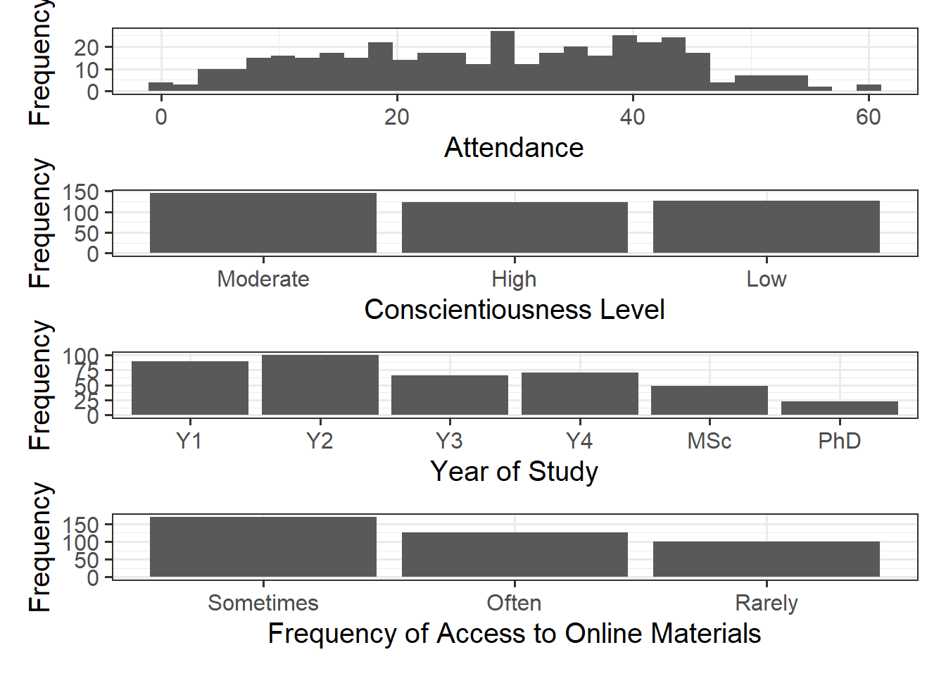
| Attendance | Total attendance (in days) |
| Conscientiousness | Conscientiousness (Levels: Low, Moderate, High) |
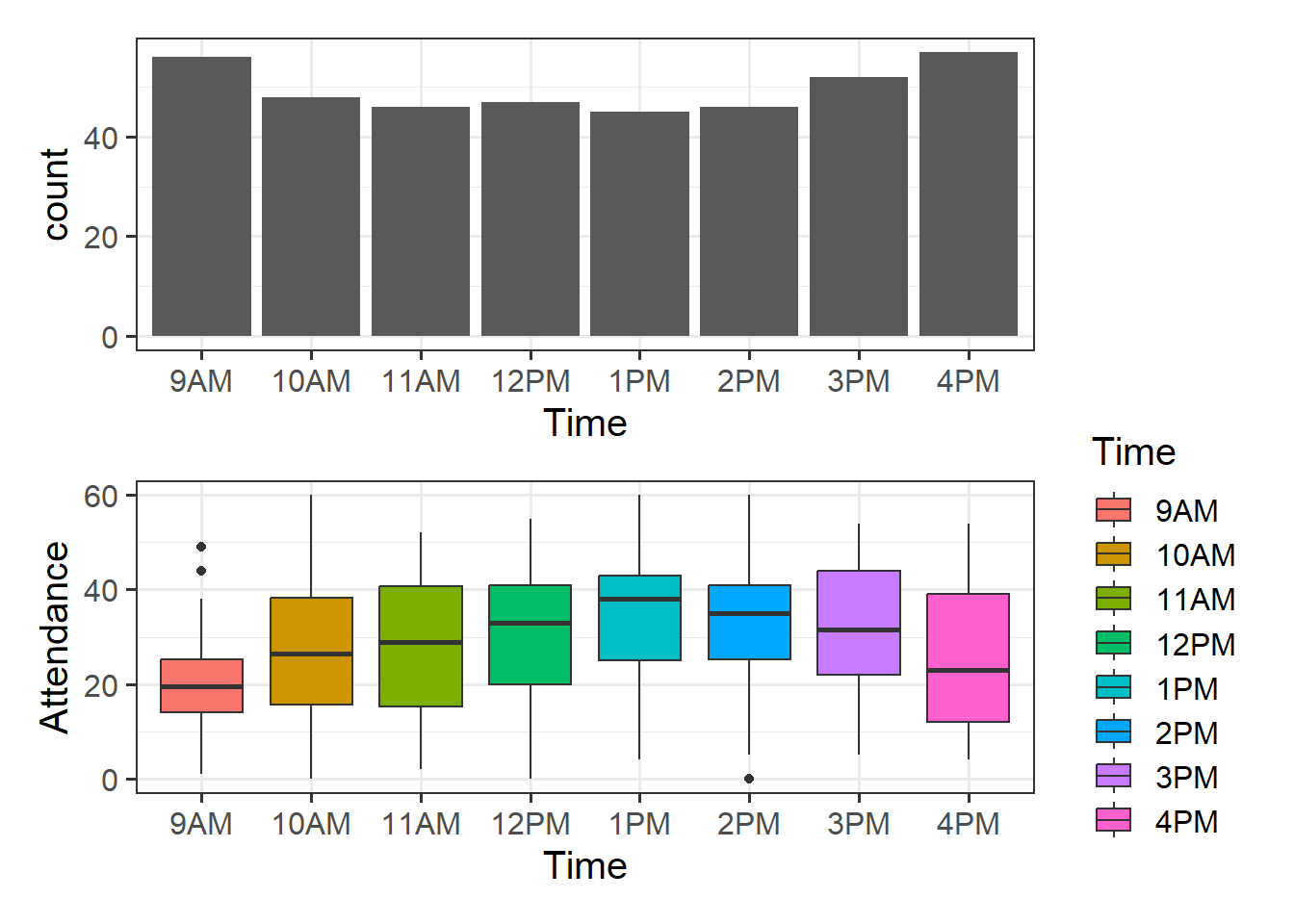
| Time | Time of Class (Levels: 9AM, 10AM, 11AM, 12PM, 1PM, 2PM, 3PM, 4PM) |
| OnlineAccess | Frequency of access to online course materials (Levels: Rarely, Sometimes, Often) |
| Year | Year of Study in University (Y1, Y2, Y3, Y4, MsC, PhD) |
Block 2 Analysis & Write-Up Example
Learning Objectives
At the end of this lab, you will:
- Understand how to write-up and provide interpretation of a linear model with multiple predictors (including categorical)
- Understand how to specify dummy and sum-to-zero coding and interpret the model output
- Understand how to specify contrasts to test specific effects
- Be able to specify and assess the assumptions underlying a linear model with multiple predictors
- Be able to assess the effect of influential cases on linear model coefficients and overall model evaluations
What You Need
- Be up to date with lectures
- Have completed Labs 7 - 10
Required R Packages
Remember to load all packages within a code chunk at the start of your RMarkdown file using library(). If you do not have a package and need to install, do so within the console using install.packages(" "). For further guidance on installing/updating packages, see Section C here.
For this lab, you will need to load the following package(s):
- tidyverse
- psych
- patchwork
- sjPlot
- kableExtra
- emmeans
- car
Lab Data
You can download the data required for this lab here and here or read the datasets in via these links https://uoepsy.github.io/data/DapR2_S1B2_PracticalPart1.csv and https://uoepsy.github.io/data/DapR2_S1B2_PracticalPart2.csv
Section A: Write-Up
In this lab you will be presented with the output from a statistical analysis, and your job will be to write-up and present the results. We’re going to use two simulated datasets based on a paper (the same two that you have worked on in lectures this week) concerning academic outcomes, student/class characteristics, and attendance.
The aim in writing should be that a reader is able to more or less replicate your analyses without referring to your R code. This requires detailing all of the steps you took in conducting the analysis. The point of using RMarkdown is that you can pull your results directly from the code. If your analysis changes, so does your report!
Make sure that your final report doesn’t show any R functions or code. Remember you are interpreting and reporting your results in text, tables, or plots, targeting a generic reader who may use different software or may not know R at all. If you need a reminder on how to hide code, format tables, etc., make sure to review the rmd bootcamp.
Important - Write-Up Examples & Plagiarism
The example write-up sections included below are not perfect - they instead should give you a good example of what information you should include within each section, and how to structure this. For example, some information is missing (e.g., description of data checks, interpretation of descriptive statistics), some information could be presented more clearly (e.g., variable names in tables, table/figure titles/captions, and rationales for choices), and writing could be more concise in places (e.g., discussion section could be more succinct and more focused on the research questions in places).
Further, you must not copy any of the write-up included below for future reports - if you do, you will be committing plagiarism, and this type of academic misconduct is taken very seriously by the University. You can find out more here.
Study Overview
Research Aim
Explore the associations among academic outcomes, student/course characteristics (e.g., class time, online access), and attendance.
Research Questions
- RQ1: Does conscientiousness, frequency of access to online materials, and year of study in University predict course attendance?
- RQ2: Is there a difference in attendance between those with early/late classes in comparison to those with midday classes?
- RQ3: Is class attendance associated with final grades?
Setup
Setup
- Create a new RMarkdown file
- Load the required package(s)
- Read the DapR2_S1B2_PracticalPart1 and DapR2_S1B2_PracticalPart2 datasets into R, assigning them to objects named
data1anddata2
Provided Analysis Code
Below you will find the code required to conduct the analysis to address the research questions. This should look similar (in most areas) to what you worked through in lecture.


The 3-Act Structure
We need to present our report in three clear sections - think of your sections like the 3 key parts of a play or story - we need to (1) provide some background and scene setting for the reader, (2) present our results in the context of the research question, and (3) present a resolution to our story - relate our findings back to the question we were asked and provide our answer.
Act I: Analysis Strategy
Question 1
Attempt to draft an analysis strategy section based on the above research question and analysis provided.
Analysis Strategy - What to Include*
Your analysis strategy will contain a number of different elements detailing plans and changes to your plan. Remember, your analysis strategy should not contain any results. You may wish to include the following sections:
- Very brief data and design description:
- Give the reader some background on the context of your write-up. For example, you may wish to describe the data source, data collection strategy, study design, number of observational units.
- Specify the variables of interest in relation to the research question, including their unit of measurement, the allowed range (e.g., for Likert scales), and how they are scored. If you have categorical data, you will need to specify the levels and coding of your variables, and what was specified as your reference level and the justification for this choice.
- Data management:
- Describe any data cleaning and/or recoding.
- Are there any observations that have been excluded based on pre-defined criteria? How/why, and how many?
- Describe any transformations performed to aid your interpretation (i.e., mean centering, standardisation, etc.).
- Model specification:
- Clearly state your hypotheses and specify your chosen significance level.
- What type of statistical analysis do you plan to use to answer the research question (e.g., simple linear regression, multiple linear regression, binary logistic regression, etc.)?
- In some cases, you may wish to include some visualisations and descriptive tables to motivate your model specification.
- Specify the model(s) to be fitted to answer your given research question and analysis structure. Clearly specify the response and explanatory variables included in your model(s). This includes specifying the type of coding scheme applied if using categorical data.
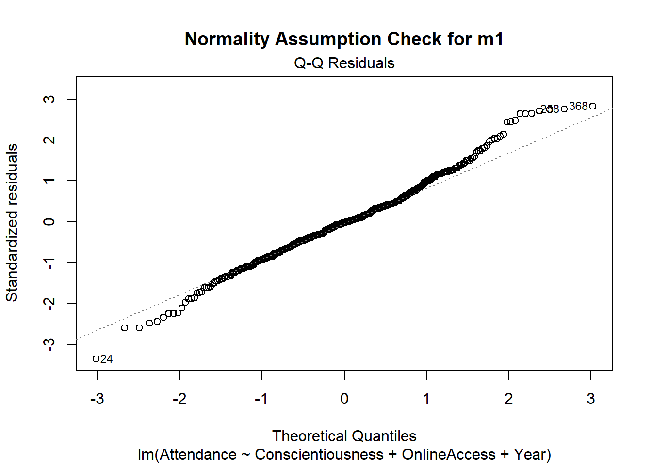
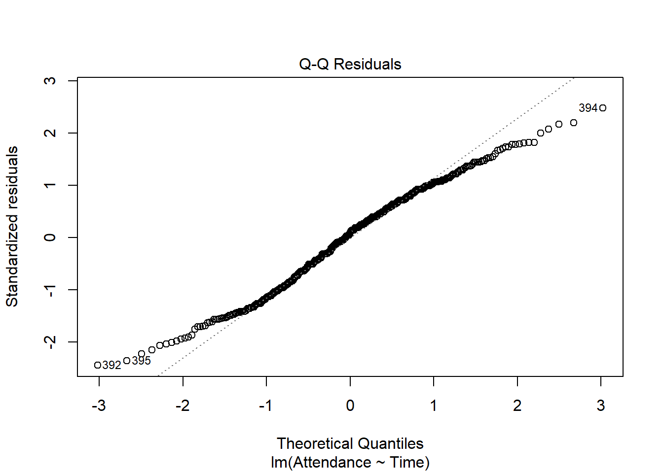
- * Specify the assumption and diagnostic checks that you will conduct. Specify what plots you will use, and how you will evaluate these.
- Note, given time constraints in lab, we have not included any reference to diagnostic checks in this write-up example - you would be expected to include this in your report. You can find more information on diagnostic checks in the S1 Week 9 Lab and S1 Week 9 Lectures.
As noted and encouraged throughout the course, one of the main benefits of using RMarkdown is the ability to include inline R code in your document. Try to incorporate this in your write up so you can automatically pull the specified values from your code. If you need a reminder on how to do this, see Lesson 3 of the Rmd Bootcamp.
Act II: Results
Question 2
Attempt to draft a results section based on your detailed analysis strategy and the analysis provided.
Results - What To Include*
The results section should follow from your analysis strategy. This is where you would present the evidence and results that will be used to answer the research questions and can support your conclusions. Make sure that you address all aspects of the approach you outlined in the analysis strategy (including the evaluation of assumptions and diagnostics).
In this section, it is useful to include tables and/or plots to clearly present your findings to your reader. It is important, however, to carefully select what is the key information that should be presented. You do not want to overload the reader with unnecessary or duplicate information (e.g., do not present print outs of the head of a dataset, or the same information in tables and plots, etc.), and you also want to save space in case there is a page limit. Make use of figures with multiple panels where you can. You can also make use of an Appendix to present your assumption and diagnostic* plots/tables, but remember that you must evaluate these in-text within the results section and clearly refer the reader to the relevant plots within the Appendix.
As a broad guideline, you want to start with the results of any exploratory data analysis, presenting tables of summary statistics and exploratory plots. You may also want to visualise associations between/among variables and report covariances or correlations. Then, you should move on to the results from your model.
- Note, given time constraints in lab, we have not included any reference to diagnostic checks in this write-up example - you would be expected to include this in your report. You can find more information on diagnostic checks in the S1 Week 9 Lab and S1 Week 9 Lectures.


Act III: Discussion
Question 3
Attempt to draft a discussion section based on your results and the analysis provided.
Discussion - What To Include
In the discussion section, you should summarise the key findings from the results section and provide the reader with a few take-home sentences drawing the analysis together and relating it back to the original question.
The discussion should be relatively brief, and should not include any statistical analysis - instead think of the discussion as a conclusion, providing an answer to the research question(s).
Assumptions & Diagnostics Appendix
Question 4
Given that the report should be kept as concise as possible, you may wish to utilize the appendix to present assumption and diagnostic plots. You must however ensure that you have:
- Described what assumptions you will check in the analysis strategy, including how you will evaluate them.
- Summarized the evaluations of your assumptions and diagnostic checks in the results section of the main report.
- Accurately referred to the figures and tables labels presented in the appendix in the main report (if you don’t refer to them, the reader won’t know what they are relevant to!).

Section B: Block 2 (Weeks 7 - 11) Recap
In the second part of the lab, there is no new content - the purpose of the recap section is for you to revisit and revise the concepts you have learned over the last 4 weeks (or the full semester if you feel that it would be beneficial to revise the materials from block 1).
We would encourage you to complete any outstanding work on these exercises (e.g., complete partial write-ups), and review solutions. Doing so will allow you to have good quality materials to refer to during the assessed report (released in Semester 2).
Given that we are now \(\frac{1}{2}\) of the way through the DAPR2 course, we would also strongly encourage you to start creating your revision materials in advance of the exam. You can access all the flashcards that you’ve been presented with in this block here. These will provide a good starting point for collating your notes together on the contents of blocks 1 & 2. We also suggest that you review your weekly quiz feedback (as many of you have learned in Psychology 2A, it is important to provide feedback to allow learners to improve their learning and retention of information, as well as correct any misunderstandings!).