| variable | description |
|---|---|
| perc_recall | The percentage of correctly recalled items |
| group | Denotes whether the individual was assigned to the roller-coaster (group = 0) or the meditation (group = 1) intervention condition |
| age | Age (in years) |
Sample Size and Power Analysis
Learning Objectives
At the end of this lab, you will:
- Understand how varying factors can influence power
- Be able to conduct power analyses using the
pwrpackage
What You Need
- Be up to date with lectures
Required R Packages
Remember to load all packages within a code chunk at the start of your RMarkdown file using library(). If you do not have a package and need to install, do so within the console using install.packages(" "). For further guidance on installing/updating packages, see Section C here.
For this lab, you will need to load the following package(s):
- tidyverse
- kableExtra
- pwr
Presenting Results
All results should be presented following APA guidelines. If you need a reminder on how to hide code, format tables/plots, etc., make sure to review the rmd bootcamp.
The example write-up sections included as part of the solutions are not perfect - they instead should give you a good example of what information you should include and how to structure this. Note that you must not copy any of the write-ups included below for future reports - if you do, you will be committing plagiarism, and this type of academic misconduct is taken very seriously by the University. You can find out more here.
Lab Data
You can download the data required for this lab here or read it in via this link https://uoepsy.github.io/data/recall_med_coast.csv
Study Overview
Research Question
Do the association between recall and age differ by intervention type?
Setup
Setup
- Create a new RMarkdown file
- Load the required package(s)
- Read in the recall_med_coast dataset into R, assigning it to an object named
recdata
Exercises
Study Overview & Data Management
Question 1
First, examine the dataset and perform any necessary and appropriate data management steps.
Next, provide a brief overview of the study design and data.
Hint
- Give the reader some background on the context of the study
- State what type of analysis you will conduct in order to address the research question
- Specify the model to be fitted to address the research question
- Specify your chosen significance (\(\alpha\)) level
- State your hypotheses
Much of the information required can be found in the Study Overview codebook.
The statistical models flashcards may also be useful to refer to. Specifically the interaction models flashcards and numeric x categorical example flashcards might be of most use.
Descriptive Statistics & Visualisations
Question 2
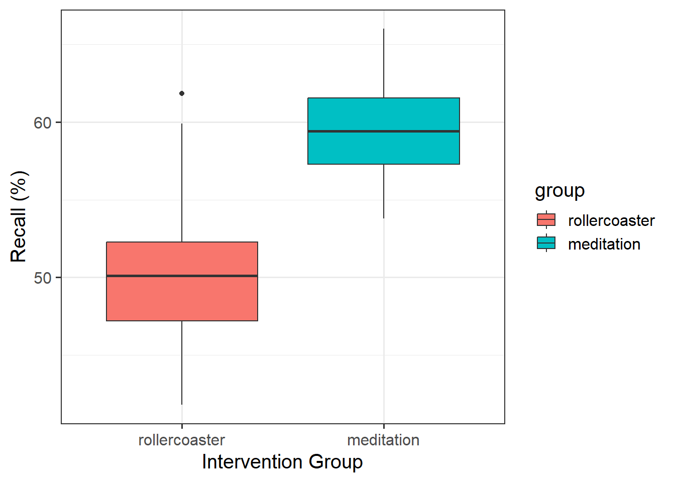
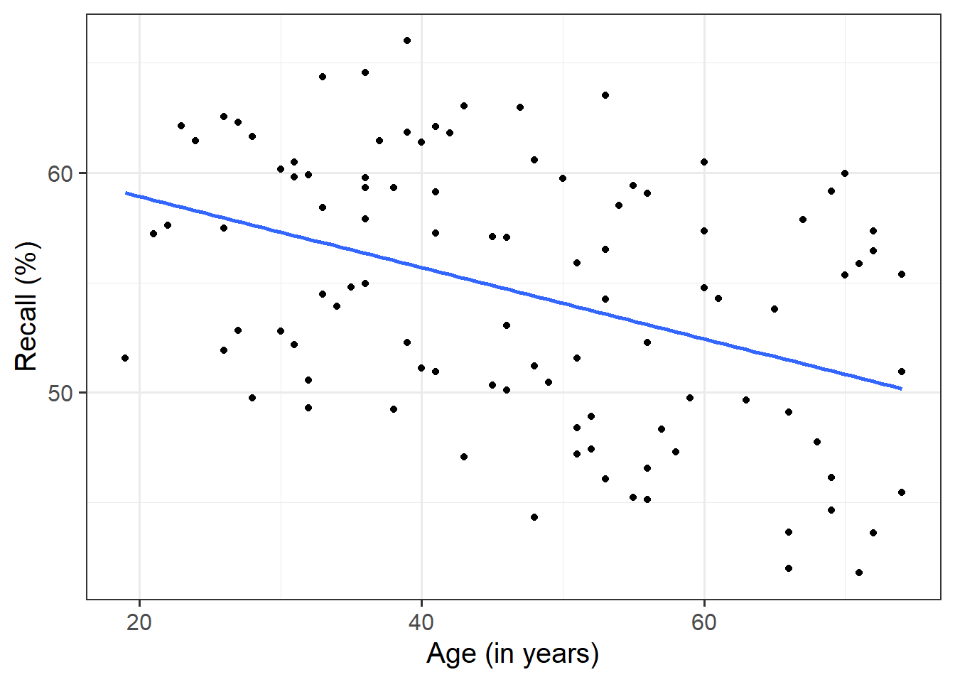
Provide a table of descriptive statistics and visualise your data.
Remember to interpret your findings in the context of the study.
Hint
Review the many ways to numerically and visually explore your data by reading over the data exploration flashcards.
For examples, see flashcards on descriptives statistics tables - categorical and numeric values examples and data visualisation - bivariate examples, paying particular attention to the type of data that you’re working with.
More specifically:
1. For your table of descriptive statistics, both the group_by() and summarise() functions will come in handy here.
- If you use the
select()function and get an error along the lines ofError in select...unused arguments..., you will need to specifydplyr::select()(this just tellsRwhich package to use the select function from).
Question 3
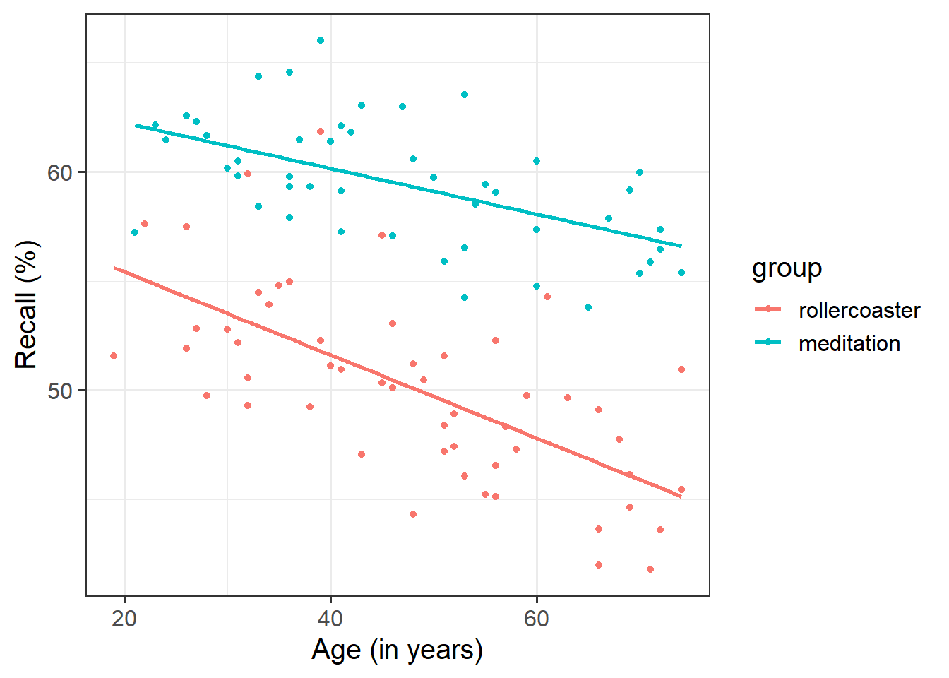
Use a scatterplot to visualise the association between recall and age by group.
Is there any evidence of an interaction between age and group?
Hint
For a recap on how to create a scatterplot, review the data visualisation - bivariate examples.
- It might be useful to specify the
color =argument for your grouping variable - Consider using
geom_smooth()to superimpose the best-fitting line describing the association of interest for each intervention group.
Sample Size & Power
Question 4
Using a significance level (\(\alpha\)) of .05, what sample size (\(n\)) would you require to check whether any of the predictors (including their interaction) influenced recall scores with a 90% chance?
Because you do not know the effect size, assume Cohen’s guideline for linear regression and, to be on the safe side, consider the ‘small’ value.
Hint
Review the following flashcards on statistical power & effect size, paying particular attention to the following two flashcards - The pwr Package and Power for Linear Regression.
Question 5
Using the same \(\alpha\) and power, what would be the sample size if you assumed effect size to be ‘medium’?
Hint
Review the following flashcards on statistical power & effect size, paying particular attention to the following two flashcards - The pwr Package and Power for Linear Regression.
Question 6
Using the same \(\alpha\) and power, what would be the sample size if you assumed effect size to be ‘large’?
Hint
Review the following flashcards on statistical power & effect size, paying particular attention to the following two flashcards - The pwr Package and Power for Linear Regression.
Question 7
Fit the following model using lm(), and assign it as an object with the name “recall_mdl1”.
\[ \text{Recall} = \beta_0 + \beta_1 \cdot \text{Age} + \epsilon \\ \]
How much variance in recall scores does the model explain?
Hint
For a recap on how to specify a simple linear model, review the statistical models flashcards.
The proportion of the total variability explained is given by \(R^2\). For a more detailed overview, see the R-squared and Adjusted R-squared flashcard.
Question 8
Imagine you found the \(R^2\) that you computed above (Q7) in a paper, and you are using that to base your next study.
A researcher believes that the inclusion of intervention group and its interaction with age should explain an extra 50% of the variation in recall scores.
Using a significance level of 5%, what sample size should you use for your next data collection in order to discover that effect with a power of 0.90?
Hint
Review the following flashcards on statistical power & effect size, paying particular attention to the following two flashcards - The pwr Package and Power for Linear Regression.
Question 9
Suppose that the aforementioned researcher made a mistake, and issues a corrected statement in which they state that the inclusion of intervention group and its interaction with age should explain an extra 5% of the variation in recall scores.
Using a significance level of 5%, what sample size should you use for your next data collection in order to discover that effect with a power of 0.90?
Hint
Review the following flashcards on statistical power & effect size, paying particular attention to the following two flashcards - The pwr Package and Power for Linear Regression.
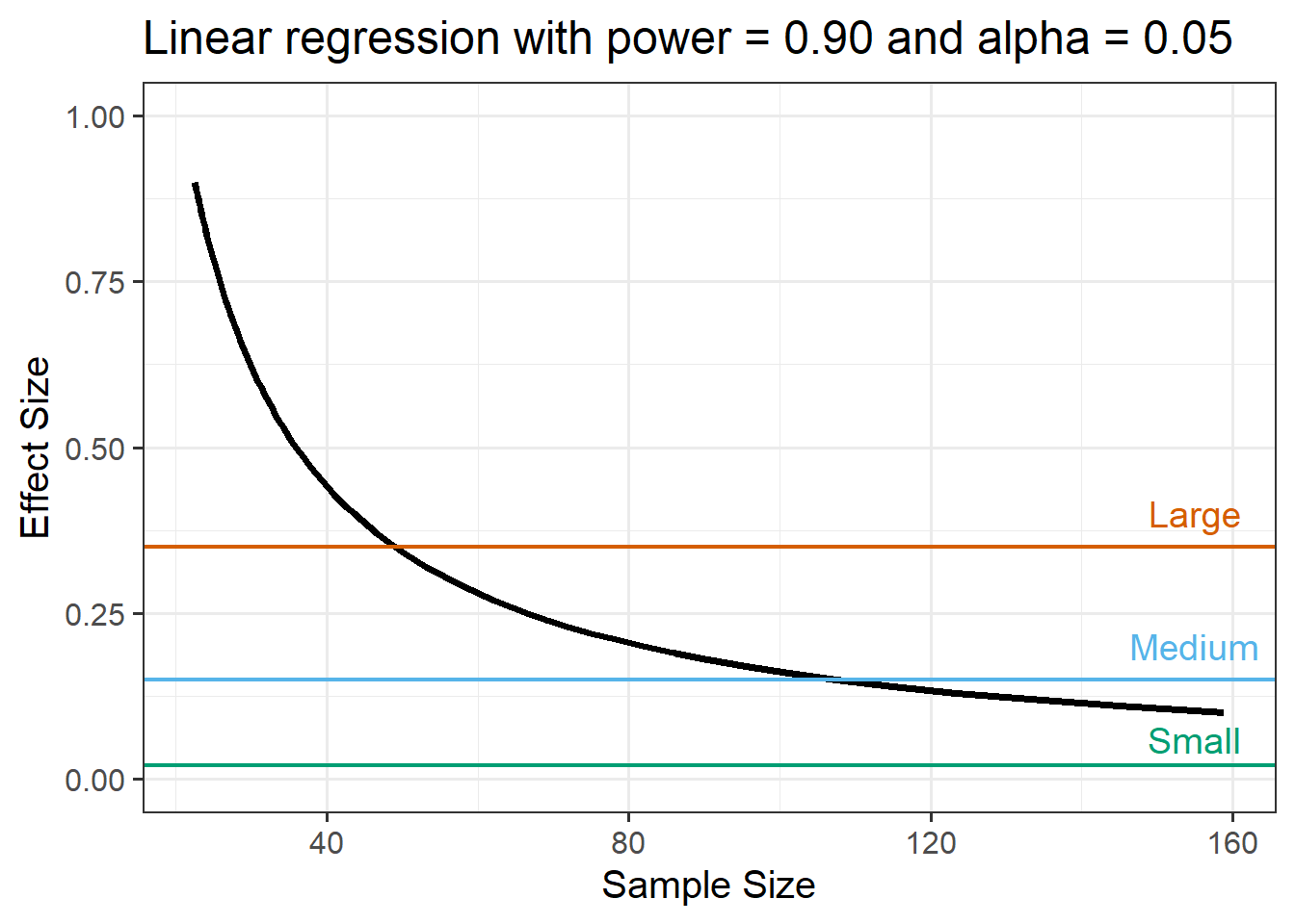
Question 10
A colleague produces a visualisation of the joint relationship between sample size and effect size via a power curve (with coloured lines representing large, medium, and small effect sizes).
Based on this, what feedback/comments might you share with them regarding sample size for their prospective study, and its relation to effect size?
Hint
Review the following flashcards on statistical power & effect size, paying particular attention to the following flashcard Factors Affecting Power.
Compile Report
Compile Report
Knit your report to PDF, and check over your work. To do so, you should make sure:
- Only the output you want your reader to see is visible (e.g., do you want to hide your code?)
- Check that the tinytex package is installed
- Ensure that the ‘yaml’ (bit at the very top of your document) looks something like this:
---
title: "this is my report title"
author: "B1234506"
date: "07/09/2024"
output: bookdown::pdf_document2
---
What to do if you cannot knit to PDF
If you are having issues knitting directly to PDF, try the following:
- Knit to HTML file
- Open your HTML in a web-browser (e.g. Chrome, Firefox)
- Print to PDF (Ctrl+P, then choose to save to PDF)
- Open file to check formatting
Hiding Code and/or Output
To not show the code of an R code chunk, and only show the output, write:
```{r, echo=FALSE}
# code goes here
```
To show the code of an R code chunk, but hide the output, write:
```{r, results='hide'}
# code goes here
```
To hide both code and output of an R code chunk, write:
```{r, include=FALSE}
# code goes here
```
Tinytex
You must make sure you have tinytex installed in R so that you can “Knit” your Rmd document to a PDF file:
install.packages("tinytex")
tinytex::install_tinytex()