Multiple Linear Regression & Standardization

Learning Objectives

At the end of this lab, you will:

  1. Extend the ideas of single linear regression to consider regression models with two or more predictors
  2. Understand how to interpret significance tests for \(\beta\) coefficients
  3. Understand how to standardize model coefficients and when this is appropriate to do
  4. Understand how to interpret standardized model coefficients in multiple linear regression models

Requirements

  1. Be up to date with lectures
  2. Have completed Week 1 and Week 2 lab exercises

Required R Packages

Remember to load all packages within a code chunk at the start of your RMarkdown file using library(). If you do not have a package and need to install, do so within the console using install.packages(" "). For further guidance on installing/updating packages, see Section C here.

For this lab, you will need to load the following package(s):

  • tidyverse
  • patchwork
  • sjPlot
  • ppcor
  • kableExtra

Presenting Results

All results should be presented following APA guidelines.If you need a reminder on how to hide code, format tables/plots, etc., make sure to review the rmd bootcamp.

The example write-up sections included as part of the solutions are not perfect - they instead should give you a good example of what information you should include and how to structure this. Note that you must not copy any of the write-ups included below for future reports - if you do, you will be committing plagiarism, and this type of academic misconduct is taken very seriously by the University. You can find out more here.

Lab Data

You can download the data required for this lab here or read it in via this link https://uoepsy.github.io/data/wellbeing_rural.csv

Study Overview

Research Question

Is there an association between wellbeing and time spent outdoors after taking into account the association between wellbeing and social interactions?

Wellbeing/Rurality data codebook.

Setup

Setup
  1. Create a new RMarkdown file
  2. Load the required package(s)
  3. Read the wellbeing dataset into R, assigning it to an object named mwdata

#Loading the required package(s)
library(tidyverse)
library(patchwork)
library(sjPlot)
library(ppcor)
library(kableExtra)

# Reading in data and storing to an object named 'mwdata'
mwdata <- read_csv("https://uoepsy.github.io/data/wellbeing_rural.csv")

Exercises

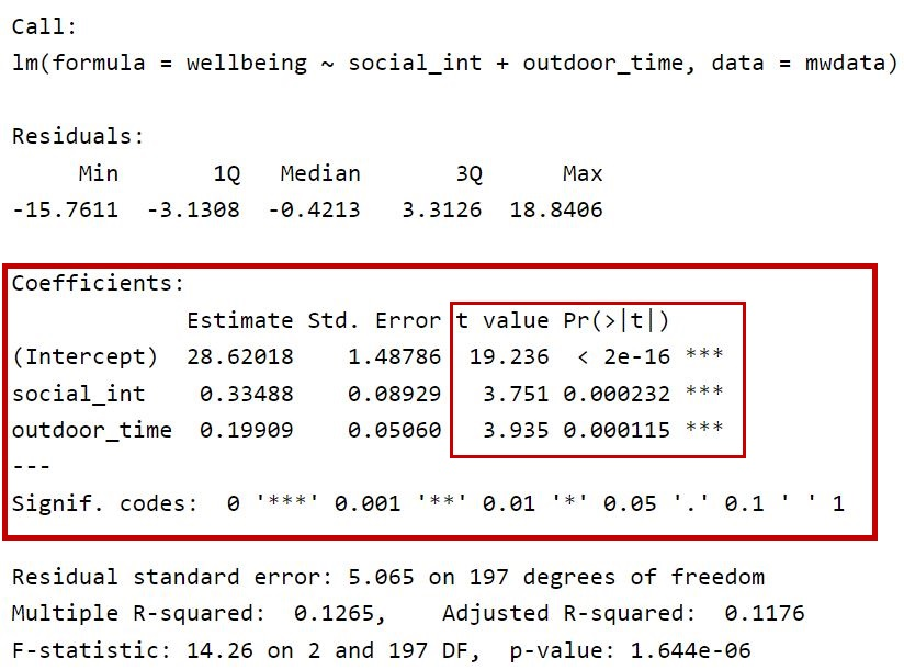
In the first section of this lab, you will focus on the statistics contained within the highlighted sections of the summary() output below. You will be both calculating these by hand and deriving via R code before interpreting these values in the context of the research question following APA guidelines. In the second section of this lab, you will focus on standardization. We will be building on last weeks lab example throughout these exercises.

Lab 2 Recap

Question 1

Fit the following multiple linear regression model, and assign the output to an object called mdl, and examine the summary output.

\[ \text{Wellbeing} = \beta_0 + \beta_1 \cdot Social~Interactions + \beta_2 \cdot Outdoor~Time + \epsilon \]

We can fit our multiple regression model using the lm() function. For a recap, see the statistical models flashcards, specifically the multiple linear regression models - description & specification card.

mdl <- lm(wellbeing ~ social_int + outdoor_time, data = mwdata)
summary(mdl)

Call:
lm(formula = wellbeing ~ social_int + outdoor_time, data = mwdata)

Residuals:
     Min       1Q   Median       3Q      Max 
-15.7611  -3.1308  -0.4213   3.3126  18.8406 

Coefficients:
             Estimate Std. Error t value Pr(>|t|)    
(Intercept)  28.62018    1.48786  19.236  < 2e-16 ***
social_int    0.33488    0.08929   3.751 0.000232 ***
outdoor_time  0.19909    0.05060   3.935 0.000115 ***
---
Signif. codes:  0 '***' 0.001 '**' 0.01 '*' 0.05 '.' 0.1 ' ' 1

Residual standard error: 5.065 on 197 degrees of freedom
Multiple R-squared:  0.1265,    Adjusted R-squared:  0.1176 
F-statistic: 14.26 on 2 and 197 DF,  p-value: 1.644e-06

Significance Tests for \(\beta\) Coefficients

Question 2

Test the hypothesis that the population slope for outdoor time is zero — that is, that there is no linear association between wellbeing and outdoor time (after controlling for the number of social interactions) in the population.

See the t value flashcard (within simple & multiple regression models - extracting Information > model coefficients > t value).

Review this weeks lecture slides for an example of how to do this by-hand and in R.

We calculate the test statistic for \(\beta_2\) as:

\[ t = \frac{\hat \beta_2 - 0}{SE(\hat \beta_2)} = \frac{0.19909 - 0}{0.05060} = 3.934585 \]

and compare it with the 5% critical value from a \(t\)-distribution with \(n-3\) degrees of freedom (since \(k = 2\), we have \(n-2-1\)), which is:

n <- nrow(mwdata)
k <- 2
tstar <- qt(0.975, df = n - k - 1)
tstar
[1] 1.972079
#tstar = 1.972079

As \(|t|\) (\(|t|\) = 3.93) is much larger than \(t^*\) (\(t^*\) = 1.97), we can reject the null hypothesis as we have strong evidence against it.

The \(p\)-value, shown below, also confirms this conclusion.

2 * (1 - pt(3.934585, n - 3))
[1] 0.0001154709

Please note that the same information was already contained in the row corresponding to the variable “outdoor_time” in the output of summary(mdl), which reported the \(t\)-statistic under t value and the \(p\)-value under Pr(>|t|):

summary(mdl)

Call:
lm(formula = wellbeing ~ social_int + outdoor_time, data = mwdata)

Residuals:
     Min       1Q   Median       3Q      Max 
-15.7611  -3.1308  -0.4213   3.3126  18.8406 

Coefficients:
             Estimate Std. Error t value Pr(>|t|)    
(Intercept)  28.62018    1.48786  19.236  < 2e-16 ***
social_int    0.33488    0.08929   3.751 0.000232 ***
outdoor_time  0.19909    0.05060   3.935 0.000115 ***
---
Signif. codes:  0 '***' 0.001 '**' 0.01 '*' 0.05 '.' 0.1 ' ' 1

Residual standard error: 5.065 on 197 degrees of freedom
Multiple R-squared:  0.1265,    Adjusted R-squared:  0.1176 
F-statistic: 14.26 on 2 and 197 DF,  p-value: 1.644e-06

The result is exactly the same (up to rounding errors) as calculating manually.

Before we interpret the results, note that sometimes \(p\)-values will be reported to \(e^X\). For example, look in the Pr(>|t|) column for “(Intercept)”. The value \(2e^{-16}\) simply means \(2 \times 10^{-16}\). This is a very small value (i.e., 0.0000000000000002), hence we would simply report it as <.001 following the APA guidelines.

We performed a \(t\)-test against the null hypothesis that outdoor time was not associated with wellbeing scores after controlling for social interactions. A significant association was found between outdoor time (hours per week) and wellbeing (WEMWBS scores) \(t(197) = 3.94,\ p < .001\), two-sided. Thus, we have evidence to reject the null hypothesis.


Question 3

Obtain 95% confidence intervals for the regression coefficients, and write a sentence about each one.

Recall the formula for obtaining a confidence interval:

A confidence interval for the population slope is \[ \hat \beta_j \pm t^* \cdot SE(\hat \beta_j) \] where \(t^*\) denotes the critical value chosen from t-distribution with \(n-k-1\) degrees of freedom (where \(k\) = number of predictors and \(n\) = sample size) for a desired \(\alpha\) level of confidence.

Review this weeks lecture slides for an example of how to do this by-hand and in R.

For 95% confidence we have \(t^* = 1.97\):

n <- nrow(mwdata)
k <- 2
tstar <- qt(0.975, df = n - k - 1)
tstar
[1] 1.972079

The confidence intervals are:

tibble(
  b0_LowerCI = round(28.62018 - (qt(0.975, n-3) * 1.48786), 3),
  b0_UpperCI = round(28.62018 + (qt(0.975, n-3)* 1.48786), 3),
  b1_LowerCI = round(0.33488 - (qt(0.975, n-3) * 0.08929), 3),
  b1_UpperCI = round(0.33488 + (qt(0.975, n-3)* 0.08929), 3),
  b2_LowerCI = round(0.19909 - (qt(0.975, n-3) * 0.05060), 3),
  b2_UpperCI = round(0.19909 + (qt(0.975, n-3)* 0.05060), 3)
      )
# A tibble: 1 × 6
  b0_LowerCI b0_UpperCI b1_LowerCI b1_UpperCI b2_LowerCI b2_UpperCI
       <dbl>      <dbl>      <dbl>      <dbl>      <dbl>      <dbl>
1       25.7       31.6      0.159      0.511      0.099      0.299

We can much more easily obtain the confidence intervals for the regression coefficients using the command confint():

confint(mdl, level = 0.95)
                   2.5 %     97.5 %
(Intercept)  25.68600170 31.5543598
social_int    0.15880045  0.5109638
outdoor_time  0.09931273  0.2988759

The result is exactly the same (up to rounding errors) as calculating manually.

  • The average wellbeing score for all those with zero hours of outdoor time and zero social interactions per week was between 25.69 and 31.55.
  • When holding weekly outdoor time constant, each increase of one social interaction per week was associated with a difference in wellbeing scores between 0.16 and 0.51, on average.
  • When holding the number of social interactions per week constant, each one hour increase in weekly outdoor time was associated with a difference in wellbeing scores between 0.1 and 0.3, on average.

Standardization

Question 4

Fit two regression models using the standardized response and explanatory variables. For demonstration purposes, fit one model using z-scored variables, and the other using the scale() function.

Both of these methods - z-scoring and scale() - will give us a standardized model.

See the scaling and standardisation flashcards.

z-score variables:

mwdata <- mwdata %>%
  mutate(
    z_wellbeing = (wellbeing - mean(wellbeing)) / sd(wellbeing),
    z_social_int = (social_int - mean(social_int)) / sd(social_int),
    z_outdoor_time = (outdoor_time - mean(outdoor_time)) / sd(outdoor_time)
  )

Check that they are standardized:

mwdata %>%
  summarise(
    M_z_wellbeing = round(mean(z_wellbeing),2), SD_z_wellbeing = sd(z_wellbeing), 
    M_z_social_int = round(mean(z_social_int),2), SD_z_social_int = sd(z_social_int),
    M_z_outdoor_time = round(mean(z_outdoor_time),2), SD_z_outdoor_time = sd(z_outdoor_time)
  )
# A tibble: 1 × 6
  M_z_wellbeing SD_z_wellbeing M_z_social_int SD_z_social_int M_z_outdoor_time
          <dbl>          <dbl>          <dbl>           <dbl>            <dbl>
1             0              1              0               1                0
# ℹ 1 more variable: SD_z_outdoor_time <dbl>
#mean of 0, SD of 1 - all good to go

Run model:

mdl_z <- lm(z_wellbeing ~ z_social_int + z_outdoor_time, data = mwdata)
mdl_s <- lm(scale(wellbeing) ~ scale(social_int) + scale(outdoor_time), data = mwdata)


Question 5

Examine the estimates from both standardized models - what do you notice?

Review the simple & multiple regression models - extracting information > model coefficients flashcards.

Consider whether the values the same, or different? What would you expect them to be and why?

summary(mdl_z)

Call:
lm(formula = z_wellbeing ~ z_social_int + z_outdoor_time, data = mwdata)

Residuals:
    Min      1Q  Median      3Q     Max 
-2.9231 -0.5806 -0.0781  0.6144  3.4942 

Coefficients:
                 Estimate Std. Error t value Pr(>|t|)    
(Intercept)    -4.168e-16  6.642e-02   0.000 1.000000    
z_social_int    2.499e-01  6.663e-02   3.751 0.000232 ***
z_outdoor_time  2.622e-01  6.663e-02   3.935 0.000115 ***
---
Signif. codes:  0 '***' 0.001 '**' 0.01 '*' 0.05 '.' 0.1 ' ' 1

Residual standard error: 0.9394 on 197 degrees of freedom
Multiple R-squared:  0.1265,    Adjusted R-squared:  0.1176 
F-statistic: 14.26 on 2 and 197 DF,  p-value: 1.644e-06
round(summary(mdl_z)$coefficients, 2)
               Estimate Std. Error t value Pr(>|t|)
(Intercept)        0.00       0.07    0.00        1
z_social_int       0.25       0.07    3.75        0
z_outdoor_time     0.26       0.07    3.93        0
summary(mdl_s)

Call:
lm(formula = scale(wellbeing) ~ scale(social_int) + scale(outdoor_time), 
    data = mwdata)

Residuals:
    Min      1Q  Median      3Q     Max 
-2.9231 -0.5806 -0.0781  0.6144  3.4942 

Coefficients:
                      Estimate Std. Error t value Pr(>|t|)    
(Intercept)         -4.106e-16  6.642e-02   0.000 1.000000    
scale(social_int)    2.499e-01  6.663e-02   3.751 0.000232 ***
scale(outdoor_time)  2.622e-01  6.663e-02   3.935 0.000115 ***
---
Signif. codes:  0 '***' 0.001 '**' 0.01 '*' 0.05 '.' 0.1 ' ' 1

Residual standard error: 0.9394 on 197 degrees of freedom
Multiple R-squared:  0.1265,    Adjusted R-squared:  0.1176 
F-statistic: 14.26 on 2 and 197 DF,  p-value: 1.644e-06
round(summary(mdl_s)$coefficients, 2)
                    Estimate Std. Error t value Pr(>|t|)
(Intercept)             0.00       0.07    0.00        1
scale(social_int)       0.25       0.07    3.75        0
scale(outdoor_time)     0.26       0.07    3.93        0

From comparing either the summary() or rounded output, we can see that the estimates are the same under both approaches. That means you can use either approach to standardize the variables in your model.


Question 6

Examine the ‘Coefficients’ section of the summary() output from the standardized and unstandardized models - what do you notice? In other words, what is the same / different?

summary(mdl)

Call:
lm(formula = wellbeing ~ social_int + outdoor_time, data = mwdata)

Residuals:
     Min       1Q   Median       3Q      Max 
-15.7611  -3.1308  -0.4213   3.3126  18.8406 

Coefficients:
             Estimate Std. Error t value Pr(>|t|)    
(Intercept)  28.62018    1.48786  19.236  < 2e-16 ***
social_int    0.33488    0.08929   3.751 0.000232 ***
outdoor_time  0.19909    0.05060   3.935 0.000115 ***
---
Signif. codes:  0 '***' 0.001 '**' 0.01 '*' 0.05 '.' 0.1 ' ' 1

Residual standard error: 5.065 on 197 degrees of freedom
Multiple R-squared:  0.1265,    Adjusted R-squared:  0.1176 
F-statistic: 14.26 on 2 and 197 DF,  p-value: 1.644e-06
round(summary(mdl)$coefficients, 2)
             Estimate Std. Error t value Pr(>|t|)
(Intercept)     28.62       1.49   19.24        0
social_int       0.33       0.09    3.75        0
outdoor_time     0.20       0.05    3.93        0
summary(mdl_z)

Call:
lm(formula = z_wellbeing ~ z_social_int + z_outdoor_time, data = mwdata)

Residuals:
    Min      1Q  Median      3Q     Max 
-2.9231 -0.5806 -0.0781  0.6144  3.4942 

Coefficients:
                 Estimate Std. Error t value Pr(>|t|)    
(Intercept)    -4.168e-16  6.642e-02   0.000 1.000000    
z_social_int    2.499e-01  6.663e-02   3.751 0.000232 ***
z_outdoor_time  2.622e-01  6.663e-02   3.935 0.000115 ***
---
Signif. codes:  0 '***' 0.001 '**' 0.01 '*' 0.05 '.' 0.1 ' ' 1

Residual standard error: 0.9394 on 197 degrees of freedom
Multiple R-squared:  0.1265,    Adjusted R-squared:  0.1176 
F-statistic: 14.26 on 2 and 197 DF,  p-value: 1.644e-06
round(summary(mdl_z)$coefficients, 2)
               Estimate Std. Error t value Pr(>|t|)
(Intercept)        0.00       0.07    0.00        1
z_social_int       0.25       0.07    3.75        0
z_outdoor_time     0.26       0.07    3.93        0

Similarities

  • The \(t\) and \(p\)-values for the two predictor variables in both models are the same. This is because the significance of these values remains the same for the standardized coefficients as for unstandardized coefficients

Differences

  • The estimates and standard errors for the intercept and both predictor variables are different under the unstandardized and standardized models
  • The \(t\) and \(p\)-values are different in each model for the intercept. This is because:
    • In the unstandardized model, the intercept is significantly different from 0 (it is 28.62), and hence has a very small \(p\)-value (< .001)
    • In the standardized model, the intercept is not significantly different from 0 (it is 0!), and hence has a \(p\)-value of 1.


Question 7

How do these standardized estimates relate to the semi-partial correlation coefficients?

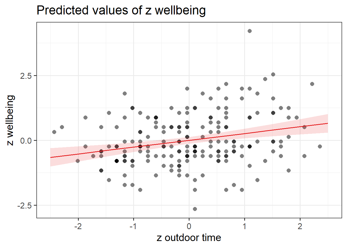
Produce a visualisation of the association between wellbeing and outdoor time, after accounting for social interactions.

Semi-partial (part) correlation coefficient

Firstly, think about what semi-partial correlation coefficients and standardized \(\beta\) coefficients represent:

  • Semi-partial correlation coefficients (which you may also see referred to as part correlations) estimate the unique contribution of each predictor variable to the explained variance in the dependent variable, while controlling for the influence of all other predictors in the model.
  • Standardized \(\beta\) estimates represent the change in the dependent variable in standard deviation units for a one-standard-deviation change in the predictor variable, whilst holding all other predictors constant.

To calculate semi-partial (part) correlation coefficients, you will need to use the spcor.test() from the ppcor package.

Recall that you can look at the estimates from either ‘mdl_s’ or ‘mdl_z’ - they contain the same standardized model estimates.

Note this is quite a difficult question (really it could be optional), and the exercise is designed to get you to think about how semi-partial correlation coefficients and standardized \(\beta\) coefficients are related.

Plotting
To visualise just one association, you need to specify the terms argument in plot_model(). Don’t forget you can look up the documentation by typing ?plot_model in the console.

Since using plot_model(), We need to use ‘mdl_z’ here not ‘mdl_s’ - it won’t work with a model that’s used the scale() function.

First, lets recall the estimates from our standardized model (rounding to 2 decimal places):

round(mdl_z$coefficients, 2)
   (Intercept)   z_social_int z_outdoor_time 
          0.00           0.25           0.26 

Next, lets calculate the semi-partial correlation coefficients:

#semi-partial (part) correlation between wellbeing & social interactions
wb_soc <- spcor.test(mwdata$wellbeing, mwdata$social_int, mwdata$outdoor_time,  method="pearson")
#round correlation coefficient estimate to 2 decimal places
round(wb_soc$estimate, 2)
[1] 0.25
#semi-partial (part) correlation between wellbeing & outdoor time
wb_out <- spcor.test(mwdata$wellbeing, mwdata$outdoor_time, mwdata$social_int, method="pearson")
#round correlation coefficient estimate to 2 decimal places
round(wb_out$estimate, 2)
[1] 0.26

We can see that the slope estimates from the standardized model are equivalent to the semi-partial (part) correlation coefficients. This makes theoretical sense given that:

In our example, we had a multiple regression model with two predictors, so in our case this means that the \(\beta^*\) coefficients quantify the change in the dependent variable when one predictor (i.e., outdoor time) changes by one standard deviation while the other predictor remains constant (i.e., number of weekly social interactions); whilst the semi-partial correlation for a given predictor (i.e., outdoor time) represents the correlation between the dependent variable and that predictor (i.e., wellbeing and outdoor time) while controlling for the other predictor (i.e., number of weekly social interactions). Thus, the standardized estimate (i.e., \(\beta^*\) coefficient) for one predictor in a multiple regression model with two predictors is equivalent to the semi-partial correlation coefficient for that predictor because, in this context, “holding all other predictors constant” refers to the one remaining predictor.

Note
If this seems a bit confusing, try not to worry - it was more a demonstration of the relationship between \(r\) and \(\beta^*\) for when you have 2 predictors (since you saw how this worked with 1 predictor in lecture, we thought it would be useful to extend to 2 predictors). Also, this can become pretty messy very quickly when you have a model with 3+ predictors as the associations among variables becomes more complex.

plot_model(mdl_z, type = "eff",
           terms = c("z_outdoor_time"), 
           show.data = TRUE)


Question 8

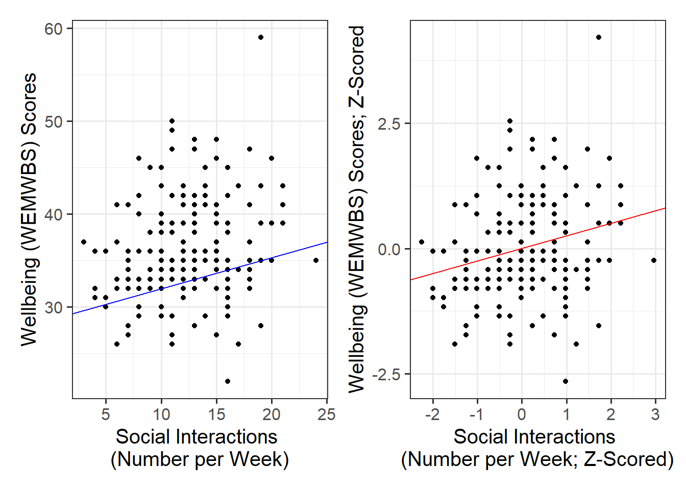
Plot the data and the fitted regression line from both the unstandardized and standardized models. To do so, for each model:

  • Extract the estimated regression coefficients e.g., via betas <- coef(mdl)
  • Extract the first entry of betas (i.e., the intercept) via betas[1]
  • Extract the second entry of betas (i.e., the slope) via betas[2]
  • Provide the intercept and slope to the function

Note down what you observe from the plots - what is the same / different?

This is very similar to Lab 1 Q7.

Extracting values
The function coef() returns a vector (a sequence of numbers all of the same type). To get the first element of the sequence you append [1], and [2] for the second.

Plotting
In your ggplot(), you will need to specify geom_abline(). This might help get you started:

geom_abline(intercept = intercept, slope = slope)


You may also want to plot these side by side to more easily compare, so consider using | from patchwork. For further ggplot() guidance, see the how to visualise data flashcard.

First extract the values required for both non-standardized and standardized models:

#non-standardized (from 'mdl')
betas <- coef(mdl)
intercept <- betas[1]
slope <- betas[2]

#standardized (from 'mdl_z')
betas_z <- coef(mdl_z)
intercept_z <- betas_z[1]
slope_z <- betas_z[2]

We can plot the models as follows:

p1 <- ggplot(data = mwdata, aes(x = social_int, y = wellbeing)) +
  geom_point() +
  geom_abline(intercept = intercept, slope = slope, color = 'blue') + 
  labs(x = "Social Interactions \n(Number per Week)", y = "Wellbeing (WEMWBS) Scores")

p2 <- ggplot(data = mwdata, aes(x = z_social_int, y = z_wellbeing)) +
  geom_point() +
  geom_abline(intercept = intercept_z, slope = slope_z, color = 'red') + 
  labs(x = "Social Interactions \n(Number per Week; Z-Scored)", y = "Wellbeing (WEMWBS) Scores; Z-Scored")

p1 | p2

Similarities

  • The data points are distributed in the same pattern
  • The slope of the line follows the same gradient

Differences

  • The x- and y-axis scales are different for each plot. This is because:
    • The unstandardized is in the original units where we interpret the slope as the change in \(y\) units for a unit change in \(x\)
    • The standardized is in SD units where we interpret the slope as the SD change in \(y\) for 1 SD change in \(x\)

Writing Up & Presenting Results

Question 9

Provide key model results from the standardized model in a formatted table.

Use tab_model() from the sjPlot package. For a quick guide, review the tables flashcard.

Since using tab_model(), We need to use ‘mdl_z’ here not ‘mdl_s’ - it won’t work with a model that’s used the scale() function.

tab_model(mdl_z,
          dv.labels = "Wellbeing (WEMWBS Scores)",
          pred.labels = c("z_social_int" = "Social Interactions (number per week)",
                          "z_outdoor_time" = "Outdoor Time (hours per week)"),
          title = "Regression Results for Wellbeing Model (both DV and IVs z-scored)")
Table 1: Regression Results for Wellbeing Model (both DV and IVs z-scored)
Regression Results for Wellbeing Model (both DV and IVs z-scored)
  Wellbeing (WEMWBS Scores)
Predictors Estimates CI p
(Intercept) -0.00 -0.13 – 0.13 1.000
Social Interactions
(number per week)
0.25 0.12 – 0.38 <0.001
Outdoor Time (hours per
week)
0.26 0.13 – 0.39 <0.001
Observations 200
R2 / R2 adjusted 0.126 / 0.118


Question 10

Interpret the results from the standardized model the context of the research question.

Make reference to the your regression table.

Remember to inform the reader of the scale of your variables.

A multiple regression model was used to determine if there was an association between well-being and time spent outdoors after taking into account the association between well-being and social interactions. All variables (wellbeing, social interactions, and outdoor time) were \(z\)-scored. As presented in Table 1, outdoor time was significantly associated with wellbeing scores \((\beta = 0.26, SE = 0.07, p < .001)\) after controlling for the number of weekly social interactions. Results suggested that, holding constant social interactions, for every standard deviation increase in outdoor time, wellbeing scores increased on average by 0.26 standard deviations. Therefore, we should reject the null hypothesis since \(p < .05\).

Compile Report

Compile Report

Knit your report to PDF, and check over your work. To do so, you should make sure:

  • Only the output you want your reader to see is visible (e.g., do you want to hide your code?)
  • Check that the tinytex package is installed
  • Ensure that the ‘yaml’ (bit at the very top of your document) looks something like this:
---
title: "this is my report title"
author: "B1234506"
date: "07/09/2024"
output: bookdown::pdf_document2
---

If you are having issues knitting directly to PDF, try the following:

  • Knit to HTML file
  • Open your HTML in a web-browser (e.g. Chrome, Firefox)
  • Print to PDF (Ctrl+P, then choose to save to PDF)
  • Open file to check formatting

To not show the code of an R code chunk, and only show the output, write:

```{r, echo=FALSE}
# code goes here
```

To show the code of an R code chunk, but hide the output, write:

```{r, results='hide'}
# code goes here
```

To hide both code and output of an R code chunk, write:

```{r, include=FALSE}
# code goes here
```

You must make sure you have tinytex installed in R so that you can “Knit” your Rmd document to a PDF file:

install.packages("tinytex")
tinytex::install_tinytex()

You should end up with a PDF file. If you have followed the above instructions and still have issues with knitting, speak with a Tutor.