Effects Coding

Learning Objectives

At the end of this lab, you will:

Understand how to specify sum-to-zero coding
Interpret the output from a model using sum-to-zero coding
Understand how to specify contrasts to test specific effects

What You Need

Be up to date with lectures
Have completed Week 7 lab exercises

Required R Packages

Remember to load all packages within a code chunk at the start of your RMarkdown file using library(). If you do not have a package and need to install, do so within the console using install.packages(" "). For further guidance on installing/updating packages, see Section C here.

For this lab, you will need to load the following package(s):

tidyverse
psych
kableExtra
emmeans

Presenting Results

All results should be presented following APA guidelines.If you need a reminder on how to hide code, format tables/plots, etc., make sure to review the rmd bootcamp.

The example write-up sections included as part of the solutions are not perfect - they instead should give you a good example of what information you should include and how to structure this. Note that you must not copy any of the write-ups included below for future reports - if you do, you will be committing plagiarism, and this type of academic misconduct is taken very seriously by the University. You can find out more here.

Lab Data

You can download the data required for this lab here or read it in via this link https://uoepsy.github.io/data/RestaurantSpending.csv

Study Overview

Research Question

Does background music in a restaurant influence the amount of money that diners spend on their meal?

A group of researchers wanted to test the claims reported in North, Shilcock, & Hargreaves (2003) on whether background music playing in a restaurant influences the amount of money diners spent on their meal.

The group of researchers got in touch with a local restaurant and asked them to alternate silence, popular music, and classical music on successive nights over 18 days. On those nights they recorded the average spend per person for each table.

In addition to the above research question, the researchers were also interested in the following:

Comparisons

Whether having some kind of music as opposed to no music (i.e., silence), resulted in a difference in the average amount of money spent by diners on their meal.

Restaurant Spending Codebook

variable	description
id	identifier for each diner
type	which one of three types of music was played (classical, pop, or none)
amount	average restaurant spending per person (in pounds - £)

id	type	amount
1	No Music	23.14891
2	Pop Music	20.59492
3	Pop Music	19.18172
4	Pop Music	16.70237
5	Classical Music	25.91041
6	Pop Music	19.27888

Setup

Create a new RMarkdown file
Load the required package(s)
Read the Restaurant Spending dataset into R, assigning it to an object named rest_spend

Exercises

Study & Analysis Plan Overview

Question 1

Examine the dataset, and perform any necessary and appropriate data management steps.

Hint

The str() function will return the overall structure of the dataset, this can be quite handy to look at
Convert categorical variables to factors, and if needed, provide better variable names*
Label factors appropriately to aid with your model interpretations if required*
Check that the dataset is complete (i.e., are there any NA values?). We can check this using is.na()
Are scores within possible ranges (e.g., if we recorded people’s age, it would be impossible to have someone aged -31!)

*See the Overview (numeric outcomes & categorical predictors) flashcard.

Let’s have a look at the data to see what we’re working with:

#first look at dataset structure
str(rest_spend)

spc_tbl_ [360 × 3] (S3: spec_tbl_df/tbl_df/tbl/data.frame)
 $ id    : num [1:360] 1 2 3 4 5 6 7 8 9 10 ...
 $ type  : chr [1:360] "No Music" "Pop Music" "Pop Music" "Pop Music" ...
 $ amount: num [1:360] 23.1 20.6 19.2 16.7 25.9 ...
 - attr(*, "spec")=
  .. cols(
  ..   id = col_double(),
  ..   type = col_character(),
  ..   amount = col_double()
  .. )
 - attr(*, "problems")=<externalptr>

#now lets look at top 6 rows (or the head) of the dataset
head(rest_spend)

# A tibble: 6 × 3
     id type            amount
  <dbl> <chr>            <dbl>
1     1 No Music          23.1
2     2 Pop Music         20.6
3     3 Pop Music         19.2
4     4 Pop Music         16.7
5     5 Classical Music   25.9
6     6 Pop Music         19.3

#check for NAs - there are none - all FALSE
table(is.na(rest_spend))


FALSE 
 1080

Let’s start with the music ‘type’ variable. This should be coded as factor (<fctr>), but can see from above it is currently coded as a character (<chr>). Let’s fix this, and rename ‘type’ to ‘music’ and remove the word ‘music’ form the labels of the levels of the factor to avoid repetition whilst we’re at it:

rest_spend <- rest_spend %>%
    mutate(
        type = factor(type, 
                           levels = c("No Music", "Pop Music", "Classical Music"),
                           labels = c("None", "Pop", "Classical"))) %>%
        rename(music = type)

Next, let’s look at the ‘amount’ variable. Here we want to check for impossible values - i.e., cannot have a negative £ per head.

# all looks ok - min and max both positive values
describe(rest_spend$amount)

   vars   n  mean   sd median trimmed  mad   min   max range  skew kurtosis
X1    1 360 22.74 3.01  22.88   22.81 3.06 13.71 33.43 19.72 -0.19      0.2
     se
X1 0.16

All participant data was complete (no missing values), with restaurant spending per person within possible ranges. Music type was coded as a factor with three levels (none, pop, and classical).

Question 2

Provide a brief overview of the study design and data, before detailing your analysis plan to address the research question.

Hint

Give the reader some background on the context of the study
State what type of analysis you will conduct in order to address the research question
Specify the model to be fitted to address the research question (note that you will need to specify the reference level of your categorical variable)
Specify your chosen significance ($\alpha$) level
State your hypotheses

Much of the information required can be found in the Study Overview codebook. The statistical models flashcards may also be useful to refer to.

The rest_spend dataset contained information on 360 hypothetical participants who took part in an experiment examining the effect of music on customer spending in a restaurant setting. Using a between-subjects design, the researchers had one of three types of music - classical, pop, or silence - played in a restaurant over 18 successive evenings. As well as recording the type of music played during the meal, the researchers also recorded the average spend per person (in £).

All participant data was complete (no missing values), with restaurant spending per person within possible ranges. Music type was coded as a factor with three levels (none, pop, and classical).

Boxplots will be used to visualise the associations among spend per person and background music conditions. To address the research question of whether spend per person differs by background music condition, we can specify our model and coding scheme as follows:

\[ \text{Restaurant Spending} = \beta_0 + \beta_1 \cdot \text{Effect Level 1} + \beta_2 \cdot \text{Effect Level 2} + \epsilon \]

where:

\[ \text{Effect Level 1} = \begin{cases} 1 & \text{if observation is from category 1} \\ 0 & \text{if observation is from category 2} \\ -1 & \text{otherwise} \end{cases} \]

\[ \text{Effect Level 2} = \begin{cases} 0 & \text{if observation is from category 1} \\ 1 & \text{if observation is from category 2} \\ -1 & \text{otherwise} \end{cases} \]

Schematically:

\[ \begin{matrix} \textbf{Level} & \textbf{Effect Level 1} & \textbf{Effect Level 2} \\ \hline \text{None} & 1 & 0 \\ \text{Pop} & 0 & 1 \\ \text{Classical} & -1 & -1 \end{matrix} \]

Effects will be considered statistically significant at $\alpha=.05$

Our hypotheses are:

$H_0:$ All $\beta_j = 0$ (for $j = 1, 2$)

There are no differences in average spend per person based on background music conditions.

$H_1:$ At least one $\beta_j \neq 0$ (for $j = 1, 2$)

There are differences in average spend per person based on background music conditions.

Descriptive Statistics & Visualisations

Question 3

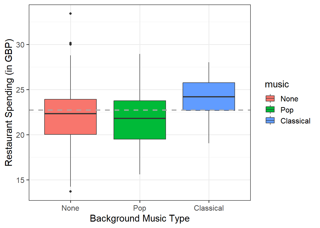
Provide a table of descriptive statistics and visualise your data.

Remember to interpret your plot in the context of the study (i.e., comment on any observed differences among treatment groups).

Hint

Review the many ways to numerically and visually explore your data by reading over the data exploration flashcards.

For examples, see flashcards on descriptives statistics tables - categorical and numeric values examples and data visualisation - bivariate examples, paying particular attention to the type of data that you’re working with.

A nice additional step you could take with your data visialisation would be to add a line representing the grand mean (the mean of all the observations). You can do this by specifying geom_hline(). Within this argument, you will need to specify where the horizontal line should cut the y-axis via yintercept =. You might want to specify line: type (via lty =), width (via lwd =), and colour (via colour =). Make sure to comment on any observed differences among the conditions in comparison to the grand mean.

Restaurant Spending & Music Type Descriptive Statistics
music	n	Mean	SD	Min	Max
None	120	22.14	3.44	13.71	33.43
Pop	120	21.90	2.97	15.60	28.94
Classical	120	24.17	1.89	19.05	28.02

Model Fitting & Interpretation

Question 4

Set the sum to zero constraint for the factor of background music.

Fit the specified model, and assign it the name “mdl_stz”.

Hint

We can switch between side-constraints using the following code:

#use dummy coding
contrasts(rest_spend$music) <- "contr.treatment"

#use sum-to-zero coding
contrasts(rest_spend$music) <- "contr.sum"

For more information, see the dummy vs effects coding flashcard.

Question 5

Interpret your coefficients in the context of the study.

Hint

Recall that under this constraint the interpretation of the coefficients becomes:

$\beta_0$ represents the grand mean
$\beta_i$ the effect due to group $i$ — that is, the mean response in group $i$ minus the grand mean

For more information, see the numeric outcomes & categorical predictors flashcards.

Coefficient	Estimate	Relation between \(\beta\) and \(\mu\)
(Intercept)	22.7382	\(\beta_0 = \frac{\mu_1 + \mu_2 + \mu_3}{3} = \mu\)
music1	-0.5968	\(\beta_1 = \mu_1 - \mu\)
music2	-0.8392	\(\beta_2 = \mu_2 - \mu\)

Question 6

Obtain the estimated (or predicted) group means for the “None,” “Pop,” and “Classical” background music conditions by using the predict() function.

Hint

Step 1: Define a data frame via tibble() with a column having the same name as the factor in the fitted model (i.e., music). Then, specify all the groups (i.e., levels) for which you would like the predicted mean.

Step 2: Pass the data frame to the predict function using the newdata = argument. The predict() function will match the column named type with the predictor called type in the fitted model ‘mdl_stz’.

If you’re still not sure, it might be helpful to review the predicted values flashcards.

Planned Comparisons / Contrasts

Question 7

Formally state the planned comparison that the researchers were interested in as a testable hypothesis.

Hint

See the manual contrasts flashcards.

Question 8

After checking the levels of the factor music, use emmeans() to obtain the estimated treatment means and uncertainties for your factor.

Hint

See the manual contrasts flashcards.

Question 9

Specify the coefficients of the comparisons and run the contrast analysis, obtaining 95% confidence intervals.

Hint

See the manual contrasts flashcards.

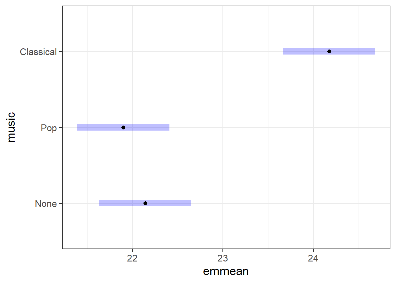
Remember that ordering matters here - look again at the output of levels(rest_spend$music) as this will help you when assigning your weights.

Question 10

Interpret the results of the contrast analysis in the context of the researchers hypotheses.

Hint

See the manual contrasts flashcards.

Compile Report

Knit your report to PDF, and check over your work. To do so, you should make sure:

Only the output you want your reader to see is visible (e.g., do you want to hide your code?)
Check that the tinytex package is installed
Ensure that the ‘yaml’ (bit at the very top of your document) looks something like this:

---
title: "this is my report title"
author: "B1234506"
date: "07/09/2024"
output: bookdown::pdf_document2
---

What to do if you cannot knit to PDF

If you are having issues knitting directly to PDF, try the following:

Knit to HTML file
Open your HTML in a web-browser (e.g. Chrome, Firefox)
Print to PDF (Ctrl+P, then choose to save to PDF)
Open file to check formatting

Hiding Code and/or Output

To not show the code of an R code chunk, and only show the output, write:

```{r, echo=FALSE}
# code goes here
```

To show the code of an R code chunk, but hide the output, write:

```{r, results='hide'}
# code goes here
```

To hide both code and output of an R code chunk, write:

```{r, include=FALSE}
# code goes here
```

Tinytex

You must make sure you have tinytex installed in R so that you can “Knit” your Rmd document to a PDF file:

install.packages("tinytex")
tinytex::install_tinytex()