Simple Linear Regression

Learning Objectives

At the end of this lab, you will:

1. Be able to specify a simple linear model
   
2. Understand what fitted values and residuals are
3. Be able to interpret the coefficients of a fitted model

Requirements

1. Be up to date with lectures
   
2. Have watched course intro video in Week 0 folder, and completed associated tasks

Required R Packages

Remember to load all packages within a code chunk at the start of your RMarkdown file using library(). If you do not have a package and need to install, do so within the console using install.packages(" "). For further guidance on installing/updating packages, see Section C here.

For this lab, you will need to load the following package(s):

• tidyverse
• sjPlot
• kableExtra

Presenting Results

All results should be presented following APA guidelines.If you need a reminder on how to hide code, format tables/plots, etc., make sure to review the rmd bootcamp.

The example write-up sections included as part of the solutions are not perfect - they instead should give you a good example of what information you should include and how to structure this. Note that you must not copy any of the write-ups included below for future reports - if you do, you will be committing plagiarism, and this type of academic misconduct is taken very seriously by the University. You can find out more here.

Lab Data

You can download the data required for this lab here or read it in via this link https://uoepsy.github.io/data/wellbeing_rural.csv

Study Overview

Research Question

Does the number of weekly social interactions influence wellbeing scores?

Wellbeing/Rurality data codebook.

Description

From the Edinburgh & Lothians, 100 city/suburb residences and 100 rural residences were chosen at random and contacted to participate in the study. The Warwick-Edinburgh Mental Wellbeing Scale (WEMWBS) was used to measure mental health and well-being.

Participants filled out a questionnaire including items concerning: estimated average number of hours spent outdoors each week, estimated average number of social interactions each week (whether on-line or in-person), whether a daily routine is followed (yes/no). For those respondents who had an activity tracker app or smart watch, they were asked to provide their average weekly number of steps.

Data Dictionary

The data in wellbeing_rural.csv contain seven attributes collected from a random sample of \(n=200\) hypothetical residents over Edinburgh & Lothians, and include:

variable	description
age	Age in years of respondent
outdoor_time	Self report estimated number of hours per week spent outdoors
social_int	Self report estimated number of social interactions per week (both online and in-person)
routine	Binary 1=Yes/0=No response to the question 'Do you follow a daily routine throughout the week?'
wellbeing	Warwick-Edinburgh Mental Wellbeing Scale (WEMWBS), a self-report measure of mental health and well-being. The scale is scored by summing responses to each item, with items answered on a 1 to 5 Likert scale. The minimum scale score is 14 and the maximum is 70
location	Location of primary residence (City, Suburb, Rural)
steps_k	Average weekly number of steps in thousands (as given by activity tracker if available)

Preview

The first six rows of the data are:

age	outdoor_time	social_int	routine	wellbeing	location	steps_k
28	12	13	1	36	rural	21.6
56	5	15	1	41	rural	12.3
25	19	11	1	35	rural	49.8
60	25	15	0	35	rural	NA
19	9	18	1	32	rural	48.1
34	18	13	1	34	rural	67.3

Setup

Setup

1. Create a new RMarkdown file
2. Load the required package(s)
3. Read the wellbeing dataset into R, assigning it to an object named mwdata

#Loading the required package(s)
library(tidyverse)
library(sjPlot)
library(kableExtra)

# Reading in data and storing to an object named 'mwdata'
mwdata <- read_csv("https://uoepsy.github.io/data/wellbeing_rural.csv")

Exercises

Marginal Distributions

Question 1

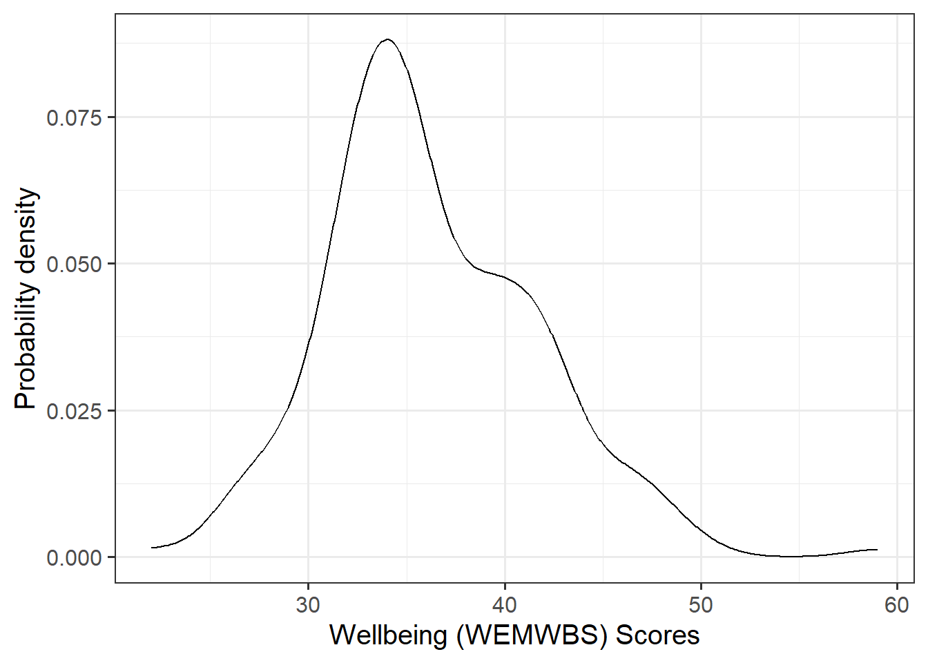
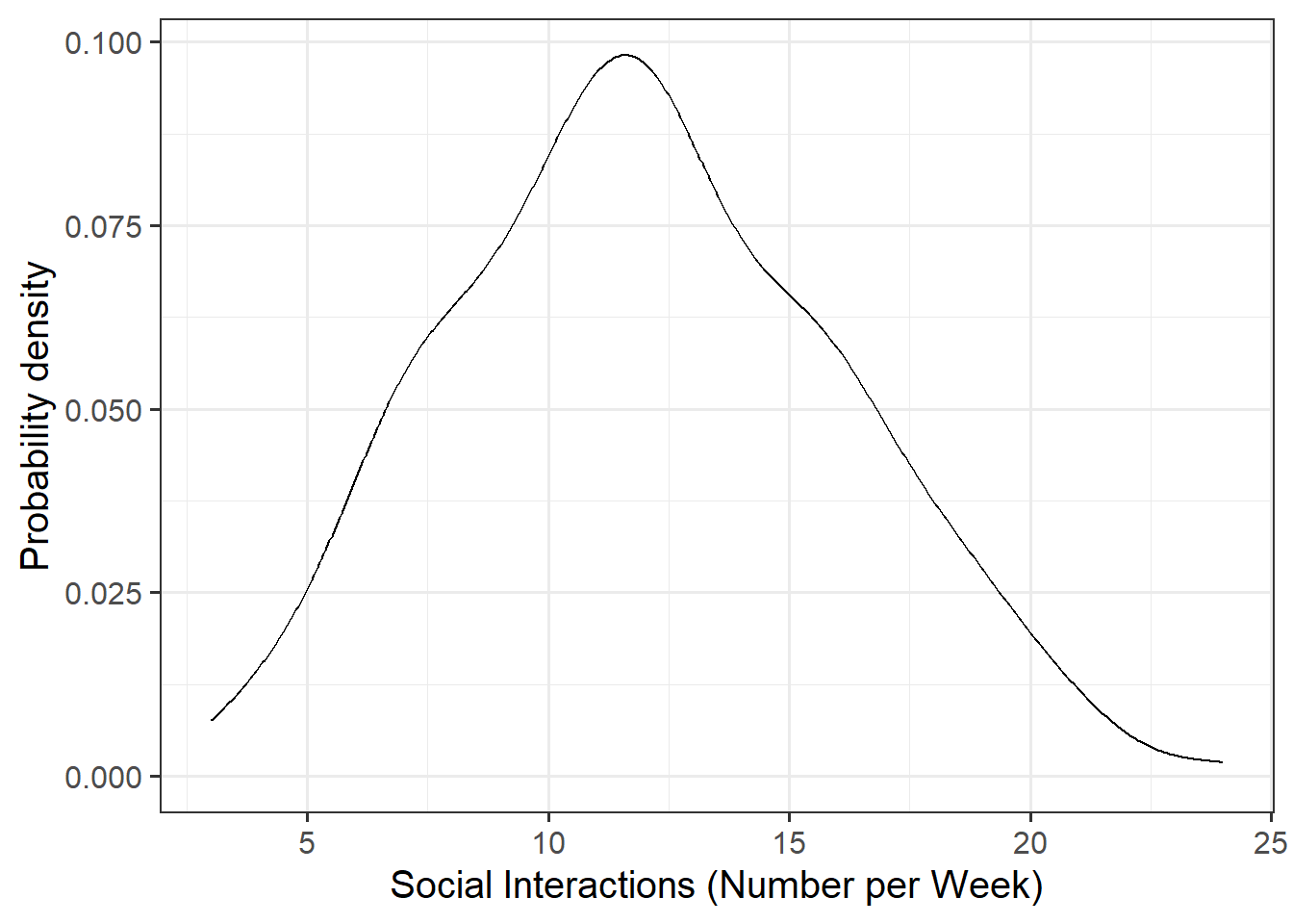
Visualise and describe the marginal distributions of wellbeing scores and social interactions.

Hint

Review the many ways to numerically and visually explore your data by reading over the data exploration flashcards.

For examples of mariginal distrubtion visualisation examples, see the data visualisation - marginal examples flashcards.

Wellbeing (WEMWBS) Scores

Visualisation of distribution:

ggplot(data = mwdata, aes(x = wellbeing)) +
  geom_density() +
  labs(x = "Wellbeing (WEMWBS) Scores", 
       y = "Probability density")

Figure 1: Distribution of Wellbeing (WEMWBS) Scores

Initial observations from plot:

• The distribution of wellbeing scores was unimodal
• Most of the wellbeing scores were between roughly 30 and 45
• The lowest wellbeing in the sample was approximately 22 and the highest approximately 59. This suggested there was a fair high degree of variation in the data
• Scores were within the range of possible values

Descriptive (or summary) statistics for wellbeing scores:

mwdata %>% 
  summarize(
    M = mean(wellbeing), 
    SD = sd(wellbeing)
    ) %>%
    kable(caption = "Wellbeing Descriptive Statistics", align = "c", digits = 2) %>%
    kable_styling(full_width = FALSE)

Table 1: Wellbeing Descriptive Statistics

Wellbeing Descriptive Statistics

M	SD
36.3	5.39

Following the exploration above, we can describe the wellbeing variable as follows:

The marginal distribution of scores on the WEMWBS was unimodal with a mean of approximately 36.3. There was variation in WEMWBS scores (SD = 5.39)

Social Interactions

Visualisation of distribution:

ggplot(data = mwdata, aes(x = social_int)) +
  geom_density() +
  labs(x = "Social Interactions (Number per Week)", 
       y = "Probability density")

Figure 2: Distribution of Number of Social Interactions

Initial observations from plot:

• The distribution of social interactions was unimodal
• Most of the participants had between 8 and 15 social interactions per week
• The fewest social interactions per week was approximately 3, and the highest approximately 24. This suggested there was a fair high degree of variation in the data

Descriptive (or summary) statistics for the number of weekly social interactions per week:

mwdata %>% 
  summarize(
    M = mean(social_int), 
    SD = sd(social_int)
    ) %>%
    kable(caption = "Social Interactions Descriptive Statistics", align = "c", digits = 2) %>%
    kable_styling(full_width = FALSE)

Table 2: Social Interactions Descriptive Statistics

Social Interactions Descriptive Statistics

M	SD
12.06	4.02

Following the exploration above, we can describe the social interactions variable as follows:

The marginal distribution of numbers of social interactions per week was unimodal with a mean of approximately 12.06. There was variation in numbers of social interactions (SD = 4.02)

Associations among Variables

Question 2

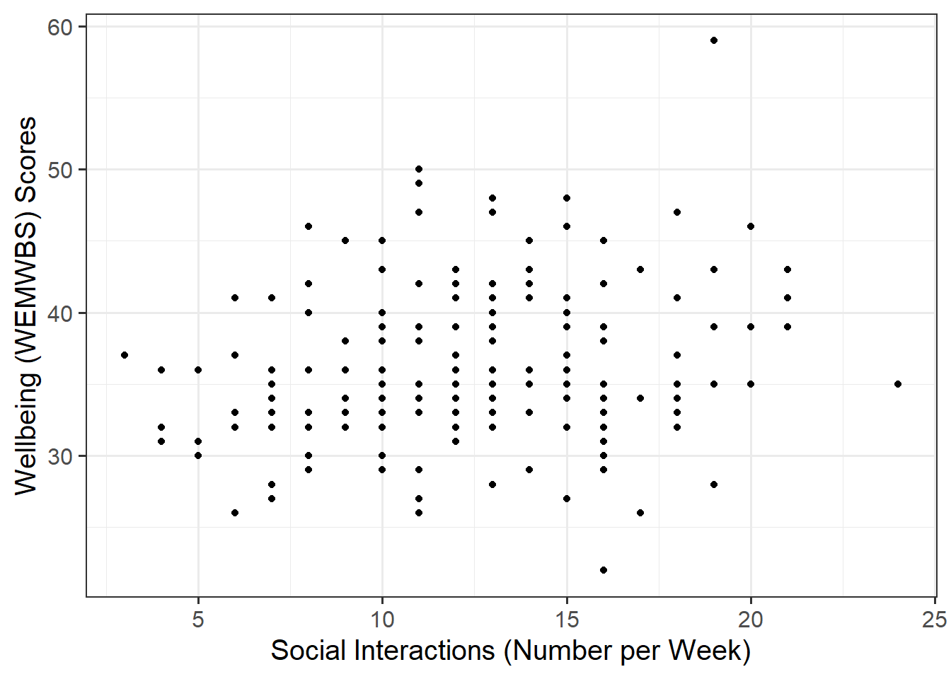
Create a scatterplot of wellbeing score and social interactions before calculating the correlation between them.

Making reference to both the plot and correlation coefficient, describe the association between wellbeing and social interactions among participants in the Edinburgh & Lothians sample.

Hint

Review the many ways to numerically and visually explore your data by reading over the data exploration flashcards.

Let’s produce a scatterplot:

ggplot(data = mwdata, aes(x = social_int, y = wellbeing)) +
  geom_point() +
  labs(x = "Social Interactions (Number per Week)", 
       y = "Wellbeing (WEMWBS) Scores")

Figure 3: Association between Wellbeing and Social Interactions

To comment on the strength of the linear association we compute the correlation coefficient in either of the following ways:

Index dataframe ([])

# correlation matrix of the two columns of interest - (check with columns we need, in this case 3 & 5)
round(cor(mwdata[,c(3,5)]), digits = 2)

           social_int wellbeing
social_int       1.00      0.24
wellbeing        0.24      1.00

Variable selection (select())

# select only the columns we want by name, and pass this to cor()
mwdata %>% 
  select(social_int, wellbeing) %>%
  cor() %>%
    round(digits = 2)

           social_int wellbeing
social_int       1.00      0.24
wellbeing        0.24      1.00

And we can see that via either method, the correlation is \[ r_{\text({Social~Interactions,~~ Wellbeing})} = .24 \]

There was a weak, positive, linear association between the weekly number of social interactions and WEMWBS scores for the participants in the sample (\(r\) = .24). More social interactions were associated, on average, with higher wellbeing scores.

Model Specification and Fitting

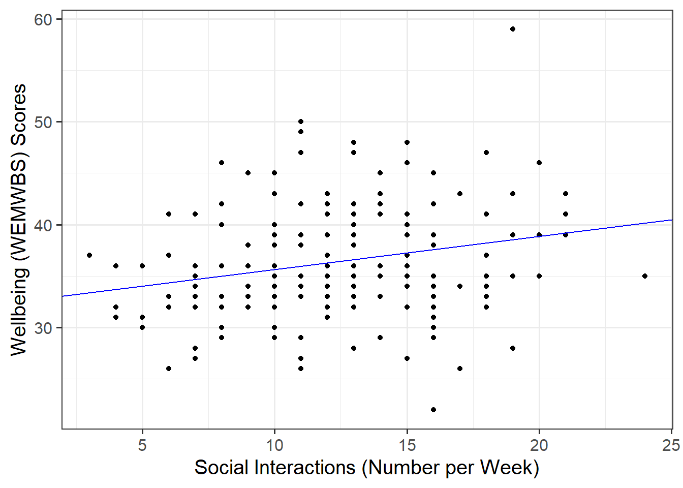
The scatterplot highlighted a linear association, where the data points were scattered around an underlying linear pattern with a roughly-constant spread as x varied.

Hence, we will try to fit a simple (i.e., one x variable only) linear regression model:

\[ y_i = \beta_0 + \beta_1 x_i + \epsilon_i \\ \quad \text{where} \quad \epsilon_i \sim N(0, \sigma) \text{ independently} \]

Question 3

First, write the equation of the fitted line.

Next, using the lm() function, fit a simple linear model to predict wellbeing (DV) by social interactions (IV), naming the output mdl.

Lastly, update your equation of the fitted line to include the estimated coefficients.

Hint

See the statistical models flashcards for a reminder on how to specify models.

For how to format and write your model in RMarkdown, see the LaTeX symbols and equations flashcard.

First, lets specify the fitted model, which can be written either as:

Option A

\[ \widehat{Wellbeing} = \hat \beta_0 + \hat \beta_1 \cdot Social~Interactions \]

Option B

\[ \widehat{Wellbeing} = \hat \beta_0 \cdot 1 + \hat \beta_1 \cdot Social~Interactions \]

To fit the model in R, as the variables are in the mwdata dataframe, we would write:

Option A

mdl <- lm(wellbeing ~ social_int, data = mwdata)
mdl

Call:
lm(formula = wellbeing ~ social_int, data = mwdata)

Coefficients:
(Intercept)   social_int  
    32.4077       0.3222  

Option B

mdl <- lm(wellbeing ~ 1 + social_int, data = mwdata)
mdl

Call:
lm(formula = wellbeing ~ 1 + social_int, data = mwdata)

Coefficients:
(Intercept)   social_int  
    32.4077       0.3222  

Note that by calling the name of the fitted model, mdl, you can see the estimated regression coefficients \(\hat \beta_0\) and \(\hat \beta_1\). We can add these values to the fitted line:

\[ \widehat{Wellbeing} = 32.41 + 0.32 \cdot Social~Interactions \\ \]

Question 4

Explore the following equivalent ways to obtain the estimated regression coefficients — that is, \(\hat \beta_0\) and \(\hat \beta_1\) — from the fitted model:

• mdl
• mdl$coefficients
• coef(mdl)
• coefficients(mdl)
• summary(mdl)

The estimated parameters returned by the below methods are all equivalent. However, summary() returns more information.

mdl

Simply invoke the name of the fitted model:

mdl

Call:
lm(formula = wellbeing ~ 1 + social_int, data = mwdata)

Coefficients:
(Intercept)   social_int  
    32.4077       0.3222  

mdl$coefficients

mdl$coefficients

(Intercept)  social_int 
 32.4077070   0.3221959 

coef(mdl)

coef(mdl)

(Intercept)  social_int 
 32.4077070   0.3221959 

coefficients(mdl)

coefficients(mdl)

(Intercept)  social_int 
 32.4077070   0.3221959 

summary(mdl)

Look under the “Estimate” column:

summary(mdl)

Call:
lm(formula = wellbeing ~ 1 + social_int, data = mwdata)

Residuals:
     Min       1Q   Median       3Q      Max 
-15.5628  -3.2741  -0.7908   3.3703  20.4706 

Coefficients:
            Estimate Std. Error t value Pr(>|t|)    
(Intercept) 32.40771    1.17532  27.573  < 2e-16 ***
social_int   0.32220    0.09243   3.486 0.000605 ***
---
Signif. codes:  0 '***' 0.001 '**' 0.01 '*' 0.05 '.' 0.1 ' ' 1

Residual standard error: 5.247 on 198 degrees of freedom
Multiple R-squared:  0.05781,   Adjusted R-squared:  0.05306 
F-statistic: 12.15 on 1 and 198 DF,  p-value: 0.0006045

The estimated intercept is \(\hat \beta_0 = 32.41\) and the estimated slope is \(\hat \beta_1 = 0.32\).

Question 5

Explore the following equivalent ways to obtain the estimated standard deviation of the errors — that is, \(\hat \sigma\) — from the fitted model mdl:

• sigma(mdl)
• summary(mdl)

The estimated standard deviation of the errors can be equivalently obtained by the below methods. However, summary() returns more information.

sigma(mdl)

sigma(mdl)

[1] 5.246982

summary(mdl)

Look at the “Residual standard error” entry of the summary(mdl) output:

summary(mdl)

Call:
lm(formula = wellbeing ~ 1 + social_int, data = mwdata)

Residuals:
     Min       1Q   Median       3Q      Max 
-15.5628  -3.2741  -0.7908   3.3703  20.4706 

Coefficients:
            Estimate Std. Error t value Pr(>|t|)    
(Intercept) 32.40771    1.17532  27.573  < 2e-16 ***
social_int   0.32220    0.09243   3.486 0.000605 ***
---
Signif. codes:  0 '***' 0.001 '**' 0.01 '*' 0.05 '.' 0.1 ' ' 1

Residual standard error: 5.247 on 198 degrees of freedom
Multiple R-squared:  0.05781,   Adjusted R-squared:  0.05306 
F-statistic: 12.15 on 1 and 198 DF,  p-value: 0.0006045

Note

The term “Residual standard error” is a misnomer, as the help page for sigma says (check ?sigma). However, it’s hard to get rid of this bad name as it has been used in too many books showing R output. For more information, check the simple & multiple regression models - extracting information flashcard flashcard.

The estimated standard deviation of the errors is \(\hat \sigma = 5.25\).

Question 6

Interpret the estimated intercept, slope, and standard deviation of the errors in the context of the research question.

Hint

To interpret the estimated standard deviation of the errors we can use the fact that about 95% of values from a normal distribution fall within two standard deviations of the center.

Intercept

The estimated wellbeing score associated with zero weekly social interactions is 32.41.

Slope

The estimated increase in wellbeing associated with one additional weekly social interaction is 0.32.

Standard deviation of the errors

For any particular number of weekly social interactions, participants’ wellbeing scores should be distributed above and below the regression line with standard deviation estimated to be \(\hat \sigma = 5.25\). Since \(2 \hat \sigma = 10.49\), we expect most (about 95%) of the participants’ wellbeing scores to be within about 11 points from the regression line.

Question 7

Plot the data and the fitted regression line. To do so:

• Extract the estimated regression coefficients e.g., via betas <- coef(mdl)
• Extract the first entry of betas (i.e., the intercept) via betas[1]
• Extract the second entry of betas (i.e., the slope) via betas[2]
• Provide the intercept and slope to the function

Hint

Extracting values
The function coef(mdl) returns a vector (a sequence of numbers all of the same type). To get the first element of the sequence you append [1], and [2] for the second.

Plotting
In your ggplot(), you will need to specify geom_abline(). This might help get you started:

geom_abline(intercept = intercept, slope = slope)

For further ggplot() guidance, see the how to visualise data flashcard.

First extract the values required:

betas <- coef(mdl)
intercept <- betas[1]
slope <- betas[2]

We can plot the model as follows:

ggplot(data = mwdata, aes(x = social_int, y = wellbeing)) +
  geom_point() +
  geom_abline(intercept = intercept, slope = slope, color = 'blue') + 
  labs(x = "Social Interactions (Number per Week)", y = "Wellbeing (WEMWBS) Scores")

Predicted Values & Residuals

Question 8

Use predict(mdl) to compute the fitted values and residuals. Mutate the mwdata dataframe to include the fitted values and residuals as extra columns.

Assign to the following symbols the corresponding numerical values:

• \(y_{3}\) (response variable for unit \(i = 3\) in the sample data)
• \(\hat y_{3}\) (fitted value for the third unit)
• \(\hat \epsilon_{5}\) (the residual corresponding to the 5th unit, i.e., \(y_{5} - \hat y_{5}\))

Hint

For a more detailed description and worked example, check the model predicted values & residuals flashcards.

mwdata_fitted <- mwdata %>%
  mutate(
    wellbeing_hat = predict(mdl),
    resid = wellbeing - wellbeing_hat
  )

head(mwdata_fitted)

# A tibble: 6 × 9
    age outdoor_time social_int routine wellbeing location steps_k wellbeing_hat
  <dbl>        <dbl>      <dbl>   <dbl>     <dbl> <chr>      <dbl>         <dbl>
1    28           12         13       1        36 rural       21.6          36.6
2    56            5         15       1        41 rural       12.3          37.2
3    25           19         11       1        35 rural       49.8          36.0
4    60           25         15       0        35 rural       NA            37.2
5    19            9         18       1        32 rural       48.1          38.2
6    34           18         13       1        34 rural       67.3          36.6
# ℹ 1 more variable: resid <dbl>

• \(y_{3}\) = 35 (see row 3, column 5)
• \(\hat y_{3}\) = 35.95 (see row 3, column 8)
• \(\hat \epsilon_{5} = y_{5} - \hat y_{5}\) = 32 - 38.21 = -6.21 (see row 5, columns 5 and 8)

Writing Up & Presenting Results

Question 9

Provide key model results in a formatted table.

Hint

Use tab_model() from the sjPlot package. For a quick guide, review the tables flashcard.

tab_model(mdl,
          dv.labels = "Wellbeing (WEMWBS) Scores",
          pred.labels = c("social_int" = "Social Interactions (Number per Week)"),
          title = "Regression Table for Wellbeing Model")

Table 3: Regression Table for Wellbeing Model

Regression Table for Wellbeing Model

	Wellbeing (WEMWBS) Scores
Predictors	Estimates	CI	p
(Intercept)	32.41	30.09 – 34.73	<0.001
Social Interactions (Number per Week)	0.32	0.14 – 0.50	0.001
Observations	200
R2 / R2 adjusted	0.058 / 0.053

Question 10

Describe the design of the study (see Study Overview codebook), and the analyses that you undertook. Interpret your results in the context of the research question and report your model results in full.

Make reference to your descriptive plots and/or statistics and regression table.

The mwdata dataset contained information on 200 hypothetical participants who lived in Edinburgh & Lothians area. Using a between-subjects design, the researchers collected information on participants’ wellbeing (measured via WEMWBS), outdoor time (hours per week), social interactions (number per week), routine (whether or not one was followed), location of residence (City, Suburb, or Rural), average weekly steps (in thousands), and age (in years).

To visualise the marginal distributions of wellbeing and social interactions, density plots were used. To understand the strength of association between the two variables, the correlation coefficient was estimated. To investigate whether the number of weekly social interactions influences wellbeing (WEMWBS) scores, the following simple linear regression model was used:

\[ \text{Wellbeing} = \beta_0 + \beta_1 \cdot \text{Social Interactions} \] From Figure 1 and Figure 2, we can see that both wellbeing \((M = 36.3, SD = 5.39)\) and social interactions \((M = 12.06, SD = 4.02)\) followed unimodal distributions. There was a weak, positive, linear association between WEMWBS scores and the weekly number of social interactions for the participants in the sample \((r = .24)\).

Full regression results are displayed in Table 3. There was a significant association between wellbeing scores and social interactions \((\beta = 0.32, SE = 0.09, p < .001)\). The estimated wellbeing score with no social interactions per week was 32.41. Each additional social interaction was associated with a 0.32 point increase in wellbeing scores.

Compile Report

Compile Report

Knit your report to PDF, and check over your work. To do so, you should make sure:

• Only the output you want your reader to see is visible (e.g., do you want to hide your code?)
• Check that the tinytex package is installed
• Ensure that the ‘yaml’ (bit at the very top of your document) looks something like this:

---
title: "this is my report title"
author: "B1234506"
date: "07/09/2024"
output: bookdown::pdf_document2
---

What to do if you cannot knit to PDF

If you are having issues knitting directly to PDF, try the following:

• Knit to HTML file
  
• Open your HTML in a web-browser (e.g. Chrome, Firefox)
  
• Print to PDF (Ctrl+P, then choose to save to PDF)
  
• Open file to check formatting

Hiding Code and/or Output

Review Lesson 5 of the rmd bootcamp for a detailed description/worked examples.

Hiding R Code

To not show the code of an R code chunk, and only show the output, write:

```{r, echo=FALSE}
# code goes here
```

Hiding R Output

To show the code of an R code chunk, but hide the output, write:

```{r, results='hide'}
# code goes here
```

Hiding R Code and Output

To hide both code and output of an R code chunk, write:

```{r, include=FALSE}
# code goes here
```

Tinytex

You must make sure you have tinytex installed in R so that you can “Knit” your Rmd document to a PDF file:

install.packages("tinytex")
tinytex::install_tinytex()

You should end up with a PDF file. If you have followed the above instructions and still have issues with knitting, speak with a Tutor.