Probabilities and log-odds

We want to model the probability with which a “success” occurs (where “success” is the standard shorthand way of talking about the level of our binary outcome which is represented as 1).

But probabilities are bounded between 0 and 1. So instead of modelling the probability of success, logistic regression models will model the log-odds of success. Log-odds are continuous and range between \(-\infty\) and \(\infty\), so they are the right kind of mathematical object that linear models can work with.

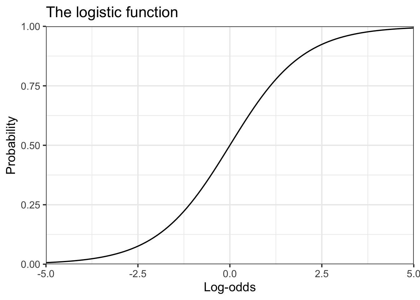
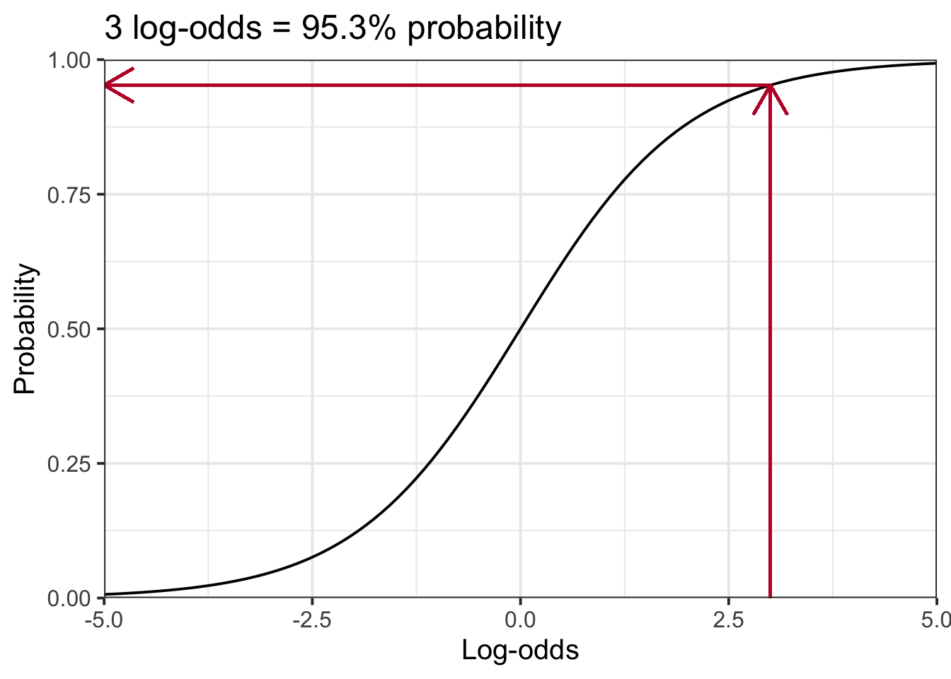
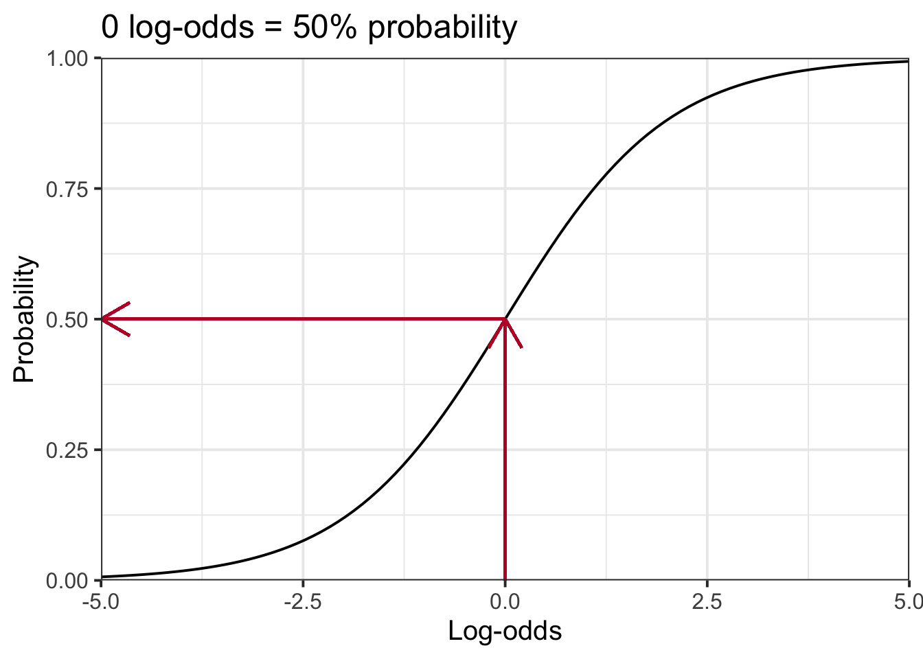
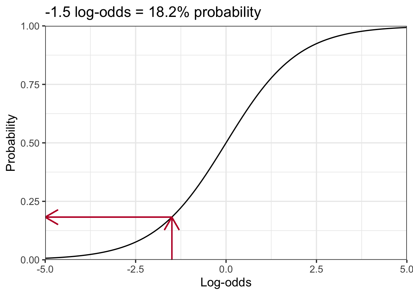
This plot shows the so-called “logistic” or “inverse logit” function, which maps log-odds to probabilities. (This function is why we call the method “logistic regression”.)

Code

p_logistic <- tibble(
  logodds = seq(-5, 5, length.out = 100),
  prob = plogis(logodds)
) |>
  ggplot(aes(x = logodds, y = prob)) +
  geom_line() +
  scale_x_continuous(expand = c(0, 0)) +
  scale_y_continuous(expand = c(0, 0), limits = c(0, 1)) +
  labs(
    y = 'Probability',
    x = 'Log-odds'
  ) +
  ggtitle('The logistic function')

p_logistic

Converting from probabilities to log-odds

The so-called logit function (logistic unit) converts probabilities to log-odds. In R, the logit function is qlogis().

For example:

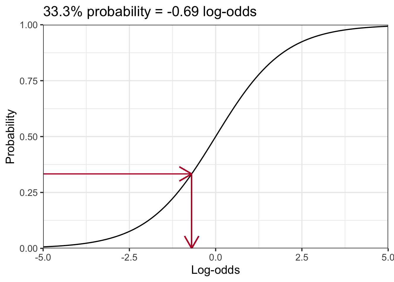
qlogis(0.333)  # 33.3% probability

[1] -0.695

Code

prob <- 0.333
p_logistic +
  # horiz
  geom_segment( x = -5, xend = qlogis(prob), y = prob, yend = prob, colour = dapr2red, arrow = arrow() ) +
  # vert
  geom_segment( x = qlogis(prob),  xend = qlogis(prob),  y = prob,  yend = 0,  colour = dapr2red, arrow = arrow() ) +
  ggtitle(paste0(prob*100, '% probability = ', round(qlogis(prob), 2), ' log-odds'))

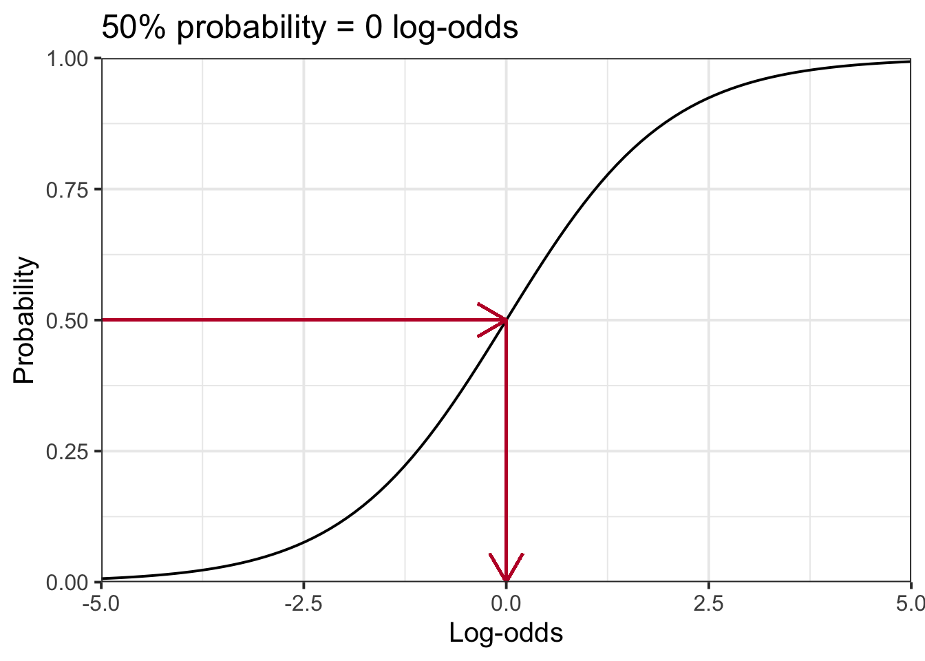
qlogis(0.5)  # 50% probability, aka 50/50 chance

[1] 0

Code

prob <- 0.5
p_logistic +
  # horiz
  geom_segment( x = -5, xend = qlogis(prob), y = prob, yend = prob, colour = dapr2red, arrow = arrow() ) +
  # vert
  geom_segment( x = qlogis(prob),  xend = qlogis(prob),  y = prob,  yend = 0,  colour = dapr2red, arrow = arrow() ) +
  ggtitle(paste0(prob*100, '% probability = ', round(qlogis(prob), 2), ' log-odds'))

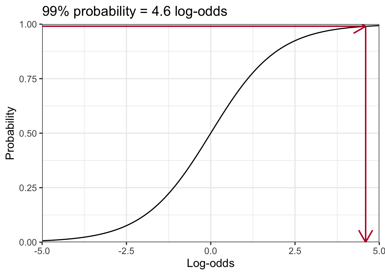
qlogis(0.99)  # 99% probability

[1] 4.6

Code

prob <- 0.99
p_logistic +
  # horiz
  geom_segment( x = -5, xend = qlogis(prob), y = prob, yend = prob, colour = dapr2red, arrow = arrow() ) +
  # vert
  geom_segment( x = qlogis(prob),  xend = qlogis(prob),  y = prob,  yend = 0,  colour = dapr2red, arrow = arrow() ) +
  ggtitle(paste0(prob*100, '% probability = ', round(qlogis(prob), 2), ' log-odds'))

Converting from log-odds to probabilities

The logistic function, aka the inverse logit function, converts log-odds to probabilities. In R, the logistic function / inverse logit function is plogis().

For example:

plogis(3)

[1] 0.953

Code

logodds <- 3

p_logistic +
  # vert
  geom_segment( x = logodds, xend = logodds, yend = plogis(logodds), y = 0, colour = dapr2red, arrow = arrow() ) +
  # horiz
  geom_segment( x = logodds,  xend = -5,  y =  plogis(logodds),  yend =  plogis(logodds),  colour = dapr2red, arrow = arrow() ) +
  ggtitle(paste0( logodds, ' log-odds = ', 100 * round(plogis(logodds), 3), '% probability'))

plogis(0)

[1] 0.5

Code

logodds <- 0

p_logistic +
  # vert
  geom_segment( x = logodds, xend = logodds, yend = plogis(logodds), y = 0, colour = dapr2red, arrow = arrow() ) +
  # horiz
  geom_segment( x = logodds,  xend = -5,  y =  plogis(logodds),  yend =  plogis(logodds),  colour = dapr2red, arrow = arrow() ) +
  ggtitle(paste0( logodds, ' log-odds = ', 100 * round(plogis(logodds), 3), '% probability'))

plogis(-1.5)

[1] 0.182

Code

logodds <- -1.5

p_logistic +
  # vert
  geom_segment( x = logodds, xend = logodds, yend = plogis(logodds), y = 0, colour = dapr2red, arrow = arrow() ) +
  # horiz
  geom_segment( x = logodds,  xend = -5,  y =  plogis(logodds),  yend =  plogis(logodds),  colour = dapr2red, arrow = arrow() ) +
  ggtitle(paste0( logodds, ' log-odds = ', 100 * round(plogis(logodds), 3), '% probability'))

The logit function is one example of a “link function”

A “link function” is what generalised linear models (GLMs) use to transform some outcome variable that’s not continuous numeric into a version that is continuous numeric, so that we can model it using a straight line.

In all the linear regression models we’ve seen in the first three blocks of DAPR2, we haven’t needed to transform the outcomes at all. You might see this written as “link function = identity”.

For logistic regression, the link function is the logit link, which transforms probabilities (bounded between 0 and 1) to log-odds (continuous numeric).

Common GLM families and their link functions

For modelling binary outcomes: the binomial family and the logit link (logistic function) or the probit link (Gaussian function).
For modelling count outcomes (i.e., integers only, like number of panic attacks in a week): the Poisson family with the log link.
For modelling positive-only numeric outcomes (e.g., reaction times): the Gamma family with the inverse link.

See ?glm for other modelling options. See ?family for other allowable link functions for each family.