library(palmerpenguins)Numeric/categorical example
RQ: Does the association between body mass and flipper length differ between species of penguin?
Here we are using the palmer penguins dataset1. The dataset contains a variety of information for a total of 344 adult penguins, including body measurements (bill length (bill_length_mm; measured in mm)/depth (bill_length_mm; measured in mm), flipper length (flipper_length_mm; measured in mm), body mass (body_mass_g; measured in grams)) for male and female (sex) penguins from three species (species; categorised as Adelie, Chinstrap, or Gentoo) across three Antarctic islands (island; categorised as Biscoe, Dream, or Torgersen) from 2007-2009 (year).
The variables that are relevant to us are body_mass_g, flipper_length_mm, and species.
Summarise/describe data
We can summarise the two continuous variables, grouped by the one categorical variable, as follows.
penguins |>
    group_by(species) |>
    summarise(
        BodyMass_M = mean(body_mass_g, na.rm = T),
        BodyMass_SD = sd(body_mass_g, na.rm = T),
        FlipperLength_M = mean(flipper_length_mm, na.rm = T),
        FlipperLength_SD = sd(flipper_length_mm, na.rm = T)
    ) |>
    kableExtra::kable(
        caption = "Descriptive statistics for body mass and flipper length in each penguin species",
        digits = 2
    ) |>
kableExtra::kable_styling(full_width = FALSE)| species | BodyMass_M | BodyMass_SD | FlipperLength_M | FlipperLength_SD |
|---|---|---|---|---|
| Adelie | 3701 | 459 | 190 | 6.54 |
| Chinstrap | 3733 | 384 | 196 | 7.13 |
| Gentoo | 5076 | 504 | 217 | 6.48 |
Visualise data
There are several options for visualising a continuous outcome variable with one continuous and one categorical predictor.
We can make a scatterplot for the two continuous variables, adding colour to distinguish the levels of each categorical variable, which will by default generate lines of best fit for each level separately.
penguins |>
  ggplot(aes(x = flipper_length_mm, y = body_mass_g, colour = species)) +
  geom_point() +
  geom_smooth(method = "lm", se = FALSE) +
  labs(x = "Flipper Length (in mm)", y = "Body Mass (in g)")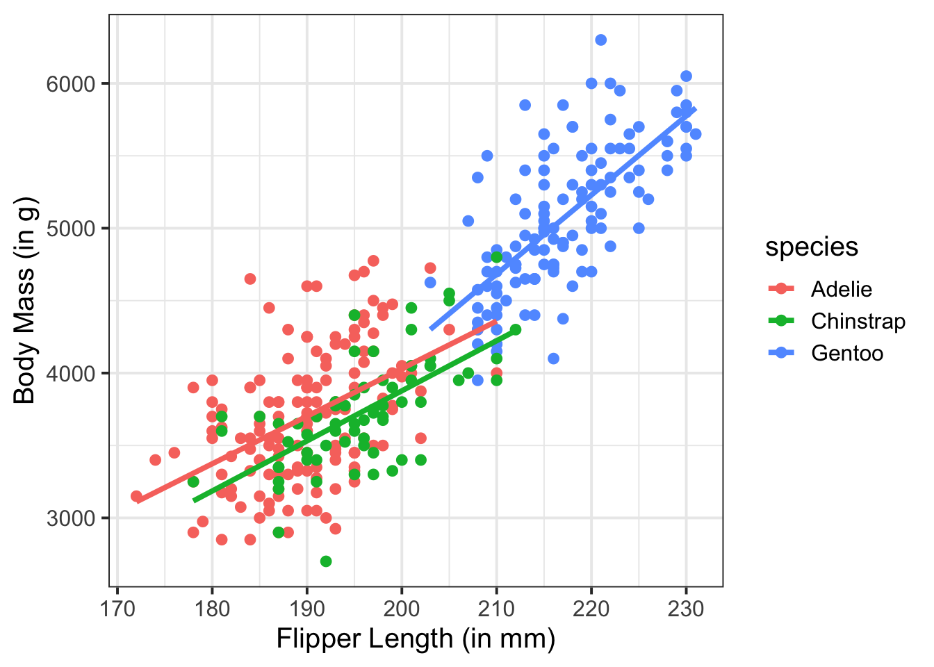
We can also distinguish the three species using facetting instead of (or in addition to) colour.
penguins |>
  ggplot(aes(x = flipper_length_mm, y = body_mass_g)) +
  geom_point() +
  facet_wrap(~species) +
  geom_smooth(method = "lm", se = FALSE) +
  labs(x = "Flipper Length (in mm)", y = "Body Mass (in g)")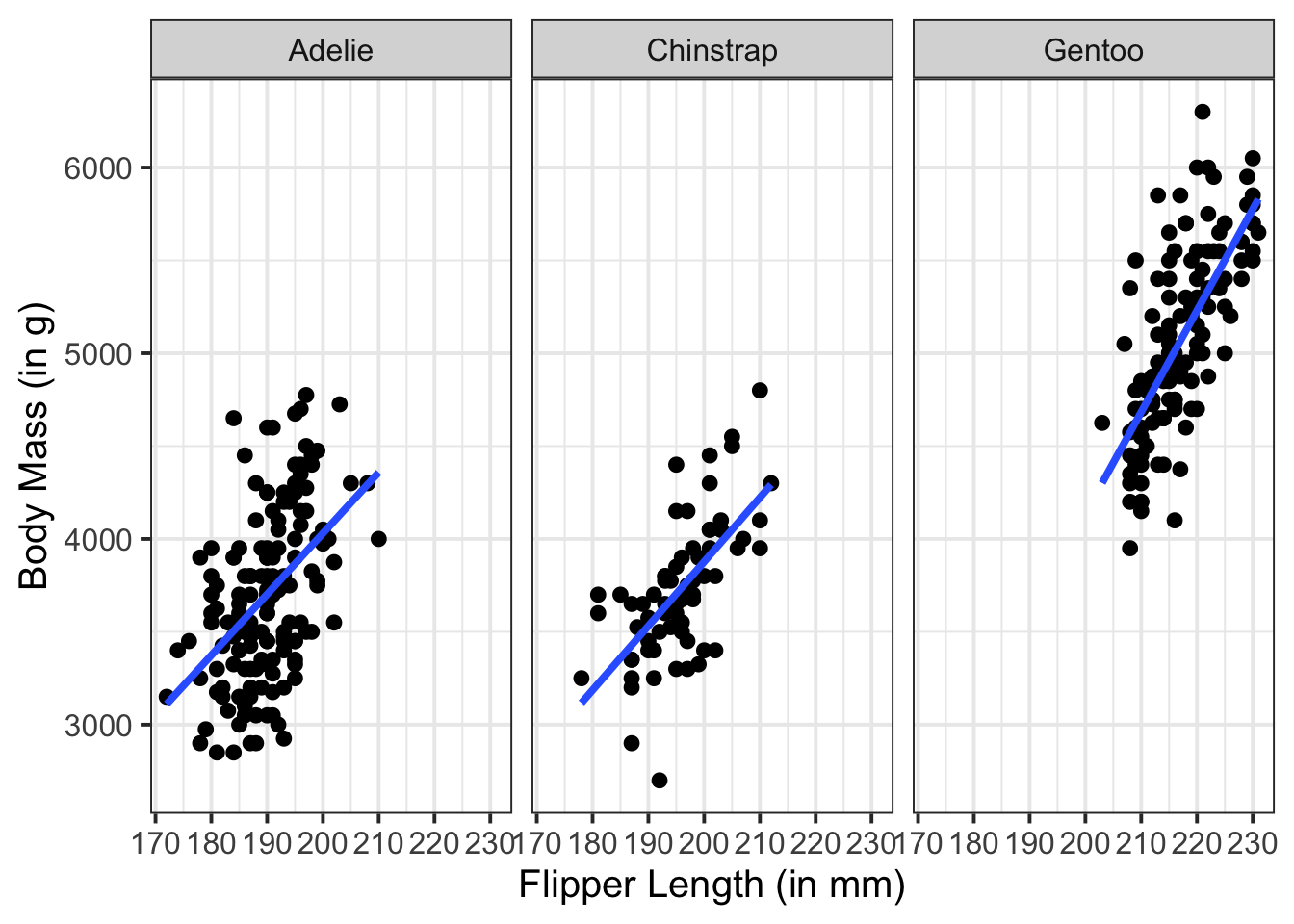
Set up predictors
Before we specify our model, we must select (and provide justification for this choice) the reference group(s) for our categorical variable(s). In this specific example, there is no natural reference category, nor one that maps to our RQ, so we will go with R’s default coding and have Adelie as our reference group for species.
contrasts(penguins$species) Chinstrap Gentoo
Adelie 0 0
Chinstrap 1 0
Gentoo 0 1The contrast matrix shows we’ll have two dummy variables, one for Chinstrap and one for Gentoo.
Next, flipper length. We could use the flipper length variable as-is, since the millimetres scale is meaningful. However, no penguins in our dataset had a flipper length of zero mm, so it might be more intuitive to mean-centre flipper_length_mm so that zero instead represents the average flipper length.
penguins <- penguins |>
  mutate(
    flipper_length_mm_c = flipper_length_mm - mean(flipper_length_mm, na.rm = T)
  )

mean(penguins$flipper_length_mm_c, na.rm=T) |> round()
[1] 0Mathematical model specification
\[ \begin{align} \text{body\_mass} ~=~ & \beta_0 + (\beta_1 \cdot \text{flipper\_length\_c}) + (\beta_2 \cdot \text{species}_\text{Chinstrap}) + (\beta_3 \cdot \text{species}_\text{Gentoo}) ~+ \\ & (\beta_4 \cdot \text{flipper\_length\_c} \cdot \text{species}_\text{Chinstrap}) ~+ \\ & (\beta_5 \cdot \text{flipper\_length\_c} \cdot \text{species}_\text{Gentoo}) + \epsilon \\ \end{align} \]
Write:
$$
\begin{align}
\text{body\_mass} ~=~ & \beta_0 + (\beta_1 \cdot \text{flipper\_length\_c}) +
(\beta_2 \cdot \text{species}_\text{Chinstrap}) +
(\beta_3 \cdot \text{species}_\text{Gentoo}) ~+ \\
& (\beta_4 \cdot \text{flipper\_length\_c} \cdot \text{species}_\text{Chinstrap}) ~+ \\
& (\beta_5 \cdot \text{flipper\_length\_c} \cdot \text{species}_\text{Gentoo}) + \epsilon \\
\end{align}
$$
H0 and H1
For most RQs that require interaction models, we’re interested in testing the hypothesis that there’s no difference in how some predictor x is associated with the outcome y for different values of z. In other words, we are interested in testing the null hypothesis that the interaction term is zero.
For the model above:
\[ \begin{align} H_0 &: \text{All } \beta_j = 0 \text{ for } j = 4, 5\\ H_1 &: \text{Any } \beta_j \neq 0\\ \end{align} \]
Write:
$$
\begin{align}
H_0 &: \text{All } \beta_j = 0 \text{ for } j = 4, 5\\
H_1 &: \text{Any } \beta_j \neq 0\\
\end{align}
$$
Fit the model
mdl_nc <- lm(body_mass_g ~ flipper_length_mm_c * species, data = penguins)Each row in the summary() output of the model will correspond to one of the estimated \(\beta\)’s in the equation above.
summary(mdl_nc)
Call:
lm(formula = body_mass_g ~ flipper_length_mm_c * species, data = penguins)

Residuals:
   Min     1Q Median     3Q    Max
-911.2 -251.9  -31.8  197.8 1144.8

Coefficients:
                                     Estimate Std. Error t value Pr(>|t|)
(Intercept)                           4060.55      59.01   68.81  < 2e-16 ***
flipper_length_mm_c                     32.83       4.63    7.10  7.7e-12 ***
speciesChinstrap                      -151.42      80.91   -1.87   0.0621 .
speciesGentoo                          126.66     108.10    1.17   0.2422
flipper_length_mm_c:speciesChinstrap     1.74       7.86    0.22   0.8247
flipper_length_mm_c:speciesGentoo       21.79       6.94    3.14   0.0018 **
---
Signif. codes:  0 '***' 0.001 '**' 0.01 '*' 0.05 '.' 0.1 ' ' 1

Residual standard error: 371 on 336 degrees of freedom
  (2 observations deleted due to missingness)
Multiple R-squared:  0.79,  Adjusted R-squared:  0.786
F-statistic:  252 on 5 and 336 DF,  p-value: <2e-16
Interpret results
\(\beta_0\) = (Intercept) = 4060.55
- An Adelie penguin with an average flipper length was expected to have a body mass of 4060.55 g.
\(\beta_1\) = flipper_length_mm_c = 32.83
- For an Adelie penguin, every 1 additional mm in flipper length was associated with a 32.83 g increase in their body mass.
- This estimate is significantly different from zero \((p < .001)\).
\(\beta_2\) = speciesChinstrap = -151.42
- A Chinstrap penguin with an average flipper length is estimated to have a body mass 151.42 g lighter than an Adelie penguin with the same flipper length.
- This estimate is not statistically different from zero \((p = .062)\).
\(\beta_3\) = speciesGentoo = 126.66
- A Gentoo penguin with an average flipper length is estimated to have a body mass 126.66g heavier than an Adelie penguin with the same flipper length.
- This estimate is not statistically different from zero \((p = .242)\).
\(\beta_4\) = flipper_length_mm_c:speciesChinstrap = 1.74
- For a Chinstrap penguin, every additional 1 mm in flipper length is associated with an additional 1.74 g increase to their body mass, compared to Adelie penguins.
- This estimate is not statistically different from zero \((p = .825)\).
\(\beta_5\) = flipper_length_mm_c:speciesGentoo = 21.79
- For a Gentoo penguin, every additional 1 mm in flipper length is associated with an additional 21.79 g increase to their body mass, compared to Adelie penguins.
- This estimate is statistically different from zero \((p = .002)\).
Visualise the model
We can do this using the probe_interaction() function from the interactions package.
In terms of of specification, it might be useful to look up the helper function (i.e., ?probe_interaction). As a quick guide:
model =: The name model to be used
pred =: The continuous predictor variable that will appear on the x-axis
modx =: The categorical moderator variable
interval =: If we sayTRUE, then confidence/prediction intervals will be plotted around the line
Remember to give your plot informative titles/labels. You, for example, likely want to give your plot:
- a clear and concise title (specify
main.title =)
- axis labels with units or scale included (specify
x.label =andy.label =)
- a legend title (specify
legend.main =)
library(interactions)

probe_mdl_nc <- probe_interaction(
  model = mdl_nc,
  pred = flipper_length_mm_c,
  modx = species,
  interval = T,
  main.title = "Predicted body mass across flipper length by species",
  x.label = "Flipper Length (in mm; mean-centered)",
  y.label = "Body mass (in g)",
  legend.main = "Penguin species"
)
probe_mdl_nc$interactplot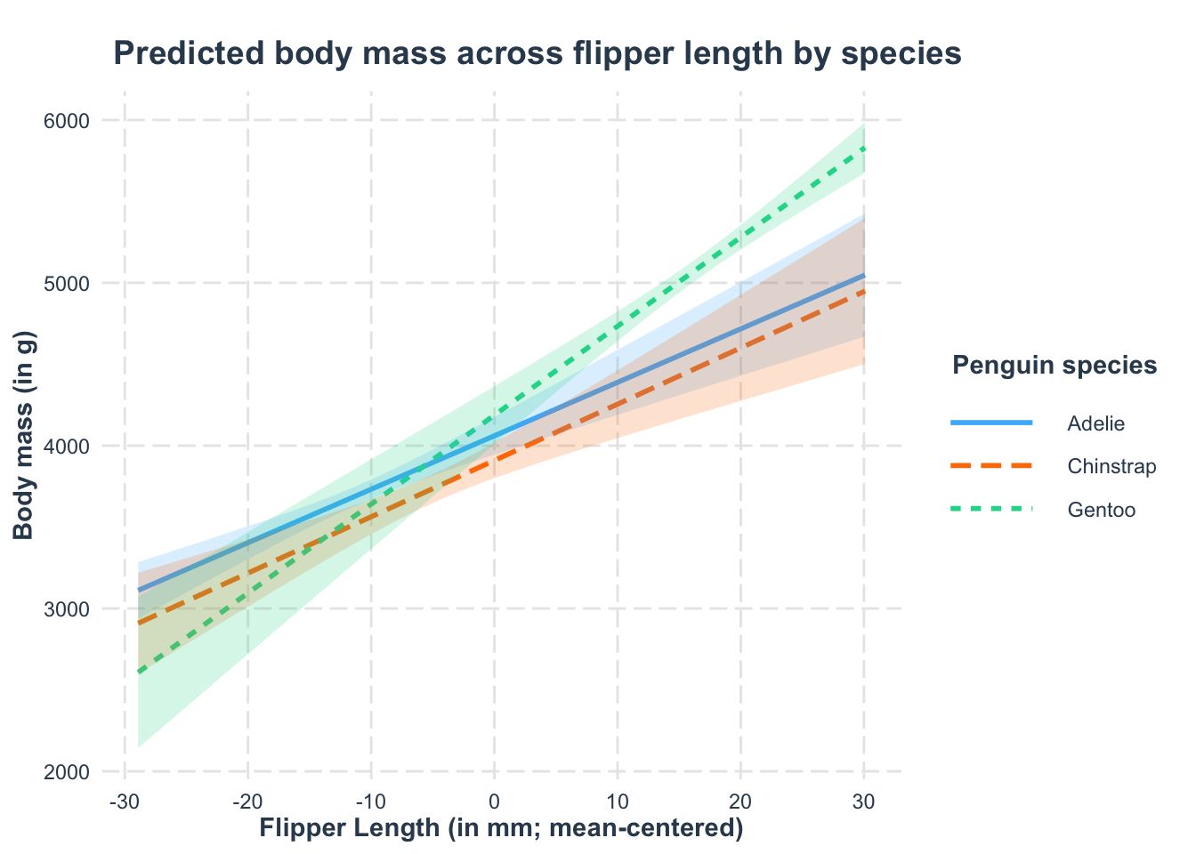
Alternatively, we can directly use the interact_plot() function and simply write
plot_mdl_nc <- interact_plot(
  model = mdl_nc,
  pred = flipper_length_mm_c,
  modx = species,
  interval = T,
  main.title = "Predicted body mass across flipper length by species",
  x.label = "Flipper Length (in mm; mean-centered)",
  y.label = "Body mass (in g)",
  legend.main = "Penguin species"
)
plot_mdl_nc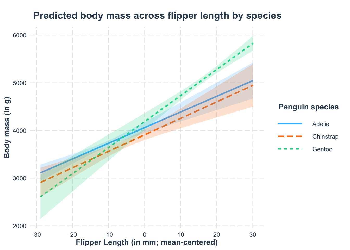
Footnotes
Horst, A. M., Hill, A. P., & Gorman, K. B. (2020). palmerpenguins: Palmer Archipelago (Antarctica) penguin data. R package version 0.1.0. https://allisonhorst.github.io/palmerpenguins/ doi: 10.5281/zenodo.3960218↩︎