recalldata <- read_csv('https://uoepsy.github.io/data/recalldata.csv')Compute model-predicted values
A note on terminology: here you will see “predicted”, “model-predicted”, “fitted”, and “model-fitted” values, and all of those mean the same thing.
Example
Imagine that you were tasked to investigate whether there was an association between recall accuracy and age. You have been provided with data from twenty participants who studied passages of text (c500 words long), and were tested a week later. The testing phase presented participants with 100 statements about the text. They had to answer whether each statement was true or false, as well as rate their confidence in each answer (on a sliding scale from 0 to 100). The dataset contains, for each participant, the percentage of items correctly answered, their age (in years), and their average confidence rating.
The data are available at https://uoepsy.github.io/data/recalldata.csv
recall_simp <- lm(recall_accuracy ~ age, data = recalldata)Model-predicted values are the estimates generated by a regression model for the dependent variable based on the independent variable(s). Residuals are the differences between these predicted values and the actual observed values (in turn indicating the accuracy of the model’s predictions).
Model-predicted values (\(\hat y_i\)) for sample data
We can get out the model-predicted values for \(y\), the “y hats” (\(\hat y\)), for the data in the sample using various functions:
predict(<fitted model>)fitted(<fitted model>)fitted.values(<fitted model>)mdl$fitted.valuesbroom::augment(<fitted model>)
For example, thie following code will give us the estimated recall accuracy (point on our regression line) for each observed value of age for each of our 20 participants.
predict(recall_simp) 1 2 3 4 5 6 7 8 9 10 11 12 13 14 15 16
62.2 73.4 69.5 68.3 70.1 71.6 58.0 66.5 66.2 77.4 65.3 71.9 69.8 68.6 73.7 72.8
17 18 19 20
72.8 68.6 71.6 66.8 These are in the same order as the observed data points, but you’d need another step to add them onto the original data frame.
A function that automatically adds model-fitted values onto the existing data frame is broom::augment() (which is to say, the augment() function from the broom package). The observed values have the same column names as in the original data frame, and the model-predicted values appear in the column .fitted.
broom::augment(recall_simp)# A tibble: 20 x 8
recall_accuracy age .fitted .resid .hat .sigma .cooksd .std.resid
<dbl> <dbl> <dbl> <dbl> <dbl> <dbl> <dbl> <dbl>
1 72 72 62.2 9.77 0.185 14.4 0.0656 0.760
2 66 35 73.4 -7.43 0.0977 14.5 0.0163 -0.549
3 47 48 69.5 -22.5 0.0502 13.5 0.0695 -1.62
4 84 52 68.3 15.7 0.0526 14.1 0.0357 1.13
5 84 46 70.1 13.9 0.0520 14.2 0.0276 1.00
6 58 41 71.6 -13.6 0.0653 14.2 0.0342 -0.989
7 52 86 58.0 -5.99 0.397 14.5 0.0968 -0.542
8 76 58 66.5 9.53 0.0712 14.4 0.0185 0.695
9 41 59 66.2 -25.2 0.0761 13.2 0.139 -1.84
10 67 22 77.4 -10.4 0.230 14.4 0.103 -0.830
11 60 62 65.3 -5.26 0.0937 14.6 0.00778 -0.388
12 67 40 71.9 -4.91 0.0694 14.6 0.00478 -0.358
13 76 47 69.8 6.21 0.0508 14.6 0.00536 0.448
14 93 51 68.6 24.4 0.0512 13.3 0.0837 1.76
15 71 34 73.7 -2.73 0.105 14.6 0.00241 -0.203
16 71 37 72.8 -1.82 0.0849 14.6 0.000830 -0.134
17 99 37 72.8 26.2 0.0849 13.1 0.172 1.92
18 66 51 68.6 -2.58 0.0512 14.6 0.000938 -0.186
19 77 41 71.6 5.39 0.0653 14.6 0.00536 0.392
20 58 57 66.8 -8.77 0.0669 14.5 0.0146 -0.638Model-predicted values for other (unobserved) data
To compute the model-predicted values for unobserved data (i.e., data not contained in the sample), we can use the following function:
predict(<fitted model>, newdata = <dataframe>)
For this example, we first need to remember that the model predicts recall_accuracy using the independent variable age. Hence, if we want predictions for new (unobserved) data, we first need to create a tibble with a column called age containing the age of individuals for which we want the prediction, and store this as a dataframe.
#Create dataframe 'newdata' containing the age values of 19, 32, and 99
newdata <- tibble(age = c(19,32,99))
newdata
# A tibble: 3 x 1
age
<dbl>
1 19
2 32
3 99Then we take newdata and add a new column called accuracy_hat, computed as the prediction from the fitted recall_simp using the newdata above:
newdata <- newdata |>
  mutate(
    accuracy_hat = predict(recall_simp, newdata = newdata)
  )
newdata
# A tibble: 3 x 2
age accuracy_hat
<dbl> <dbl>
1 19 78.3
2 32 74.3
3 99 54.1Predicted Values - Example
Lets estimate (or predict) recall accuracy of two individuals with the following ages (a) 18, and (b) 118. There are a few ways we can do this, but first, let’s recall our fitted model:
\[ \text{Recall accuracy} = 84.02 - 0.31 \cdot \text{Age} \]
Substitute in Values
- The predicted average recall accuracy for individuals who are aged 18 is:
\(84.02 - (0.31 * 18) = 78.44\)
- The predicted average recall accuracy for individuals who are aged 118 is:
\(84.02 - (0.31 * 118) = 47.44\)
Use the predict() Function
newdata <- tibble(age = c(18, 118))

accuracy_hat <- predict(recall_simp, newdata = newdata)
accuracy_hat
1 2
78.6 48.3 We can see that both approaches (manually substituting values into the regression equation or using the predict() function) both give us the same values (slightly different due to rounding).
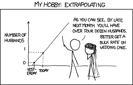
But, be careful to not go too far off the range of the available data (I don’t know many 118 year olds, do you?). If you do, you will extrapolate. This is very dangerous…