Comparing LMs

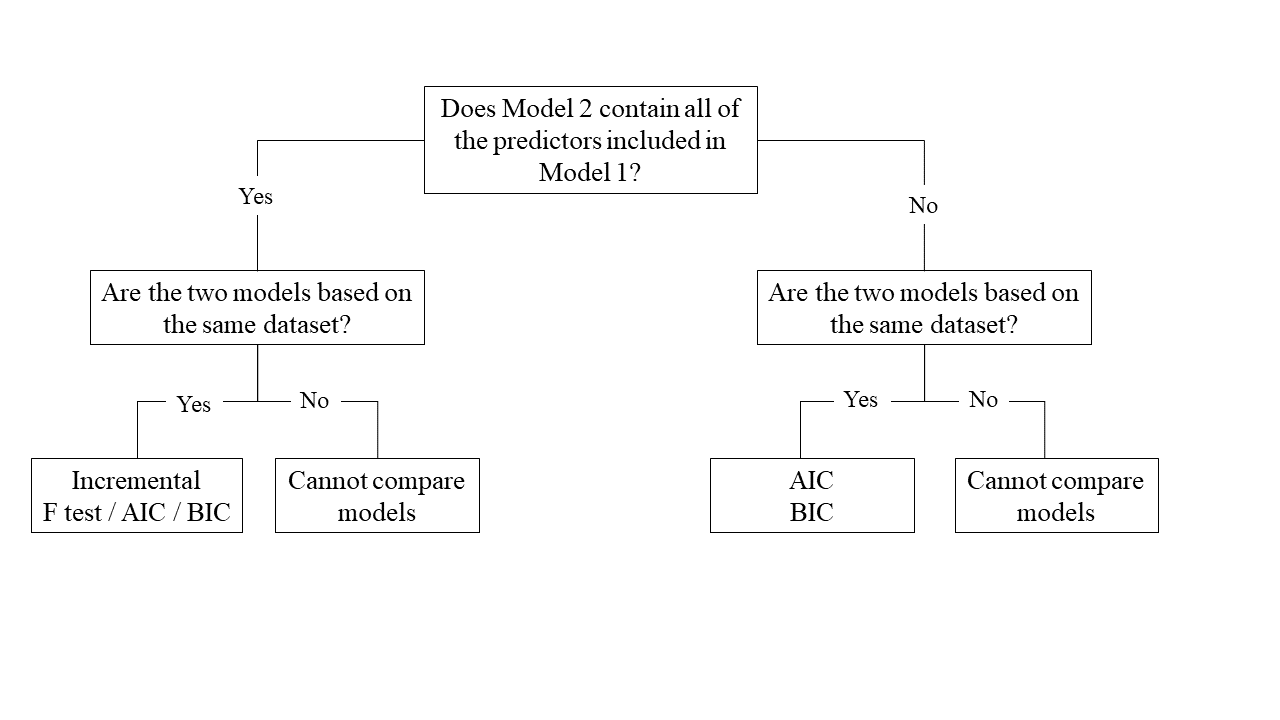
One useful thing we might want to do is compare our models with and without some predictor(s). There are numerous ways we can do this, but the method chosen depends on the models and underlying data:

Nested vs Non-Nested Models

Nested Models

Imagine you have two regression models where Model 1 contains a subset of the predictors contained in the other Model 2 and is fitted to the same data.

More simply, Model 2 contains all of the predictors included in Model 1, plus additional predictor(s).

This means that Model 1 is nested within Model 2, or that Model 1 is a submodel of Model 2.

Non-Nested Models

Imagine you have two regression models where Model 1 contains different variables to those contained in Model 2, where both models are fitted to the same data.

More simply, Model 1 and Model 2 contain unique variables that are not shared.

This means that Model 1 and Model 2 are not nested.

Incremental F-test

This is a test of whether the additional predictors provide a better fitting model.
Formally this is the test of:

\(H_0:\) coefficients for the added/omitted variables are all zero.
\(H_1:\) at least one of the added/omitted variables has a coefficient that is not zero.

The formula for the F-ratio

The \(F\)-ratio for comparing the residual sums of squares between two models can be calculated as:

\[ F_{(df_R-df_F),~df_F} = \frac{(SSR_R-SSR_F)/(df_R-df_F)}{SSR_F / df_F} \\ \quad \\ \] \[ \begin{align} & \text{Where:} \\ \\ & SSR_R = \text{residual sums of squares for the restricted model} \\ & SSR_F = \text{residual sums of squares for the full model} \\ & df_R = \text{residual degrees of freedom from the restricted model} \\ & df_F = \text{residual degrees of freedom from the full model} \\ \end{align} \]

Run the test

We can conduct an incremental \(F\)-test to compare two models by fitting both models using lm(), and passing them to the anova() function (name the smaller, nested model first):

model1 <- lm( ... )
model2 <- lm( ... )
anova(model1, model2)

Note: we are NOT running an ANOVA here. This analysis must be reported as an incremental F-test. It’s a misleading coincidence that the function in R that does this test happens to be the function called anova().

If we wanted to, for example, compare a model with just one predictor, \(x1\), to a model with 2 predictors: \(x1\), and \(x2\), we can assess the extent to which the variable \(x2\) improves model fit:

model1 <- lm(y ~ x1, data = data_name)
model2 <- lm(y ~ x1 + x2, data = data_name)
anova(model1, model2)

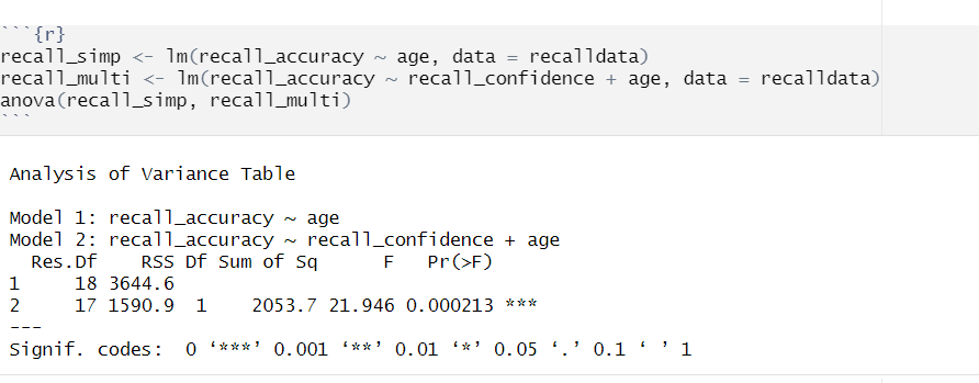
For example (this is not the best example because it compares two models differing only in one predictor, and you get the same information from that additional predictor’s significance test, but it will illustrate the process):

Report in APA format

A couple of options, depending on what exactly the RQ is asking:

Recall confidence explained a significant amount of variance in recall accuracy beyond the explanatory power of age \((F(1, 17) = 21.95, p < .001)\).
Recall accuracy is significantly predicted by recall confidence, over and above the impact of age \((F(1, 17) = 21.95, p < .001)\).

AIC & BIC

AIC (Akaike Information Criterion) and BIC (Bayesian Information Criterion) combine information about the sample size, the number of model parameters, and the residual sums of squares (\(SS_{residual}\)). Models do not need to be nested to be compared via AIC and BIC, but they need to have been fit to the same dataset.

The formulas for AIC and BIC

AIC can be calculated as:

\[ \begin{align} & AIC = n\,\text{ln}\left( \frac{SS_{residual}}{n} \right) + 2k \\ \end{align} \quad \\ \]

BIC can be calculated as:

\[ \begin{align} & BIC = n\,\text{ln}\left( \frac{SS_{residual}}{n} \right) + k\,\text{ln}(n) \\ \end{align} \quad \\ \]

Where for both AIC and BIC:

\[ \begin{align} & SS_{residual} = \text{sum of squares residuals} \\ & n = \text{sample size} \\ & k = \text{number of explanatory variables} \\ & \text{ln} = \text{natural log function} \end{align} \]

For both of these fit indices, lower values are better, and both include a penalty for the number of predictors in the model (although BIC’s penalty is harsher).

So how do we determine whether there is a statistical difference between two models? To evaluate our model comparisons, we need to look at the difference (\(\Delta\)) between the two values:

AIC: There are no specific thresholds to suggest how big a difference in two models is needed to conclude that one is substantively better than the other
BIC: Using the following \(\Delta BIC\) cutoffs (Raftery, 1995):

Value	Interpretation of Difference between Models
\(\Delta < 2\)	No evidence
\(2 > \Delta < 6\)	Positive evidence
\(6 > \Delta < 10\)	Strong evidence
\(\Delta > 10\)	Very strong evidence

Run the calculations

We can calculate AIC and BIC by using the AIC() and BIC() functions respectively:

#AIC
AIC(modelname)

#BIC
BIC(modelname)

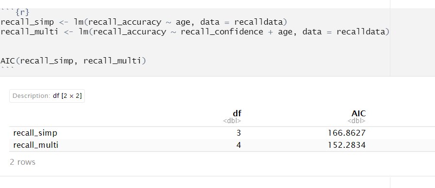
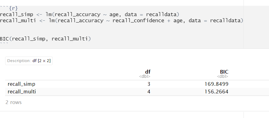
For example (again, this is not the best example because it compares two models differing only in one predictor, and you get the same information from that additional predictor’s significance test, but it will illustrate the process):

Using AIC:

and BIC:

Report in APA format

Based on both AIC and BIC, the model predicting recall accuracy that included both recall confidence and age was better fitting \((\text{AIC} = 152.28; \text{BIC} = 156.27)\) than the model with age alone \((\text{AIC} = 166.86; \text{BIC} = 169.85)\).