Deterministic functions vs. probabilistic models

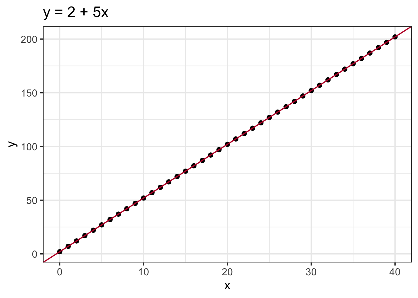
In a linear function like \(y = 2 + 5x\), every time we set \(x = 6\), this function will result in \(y = 32\). There is no variability in the outcome. The name for functions like this, where there is always the exact same relationship between input and output with no deviation, is “deterministic”. The output is determined by the input.

Code

max_x <- 40

tibble(
  x = 0:max_x,
  y = 2 + 5*x
) |>
  ggplot(aes(x = x, y = y)) +
  geom_point() +
  geom_abline(intercept = 2, slope = 5, colour = dapr2red) +
  ggtitle('y = 2 + 5x') +
  NULL

“Deterministic” is the opposite of “probabilistic” or “statistical”, where random variability can affect how \(x\) corresponds to \(y\).

To make \(y = 2 + 5x\) a statistical model, we add on another term \(\epsilon\) (the Greek letter epsilon), which represents some variability or “error”, which appears graphically as the points being some distance above or below the modelled line.

\[ y = 2 + 5x + \epsilon \]

Code

set.seed(1)
tibble(
  x = 0:max_x,
  error = rnorm(max_x+1, 0, 20),
  y = 2 + (5*x) + error
) |>
  ggplot(aes(x = x, y = y)) +
  geom_point() +
  geom_abline(intercept = 2, slope = 5, colour = dapr2red) +
  ggtitle('y = 2 + 5x + epsilon') +
  NULL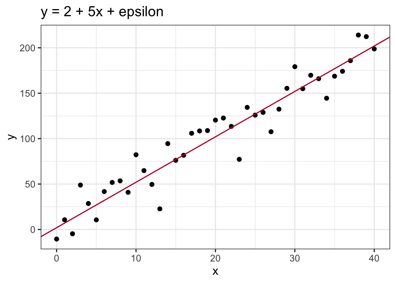

Now if we set \(x = 6\), \(y\) is equal to \(32 + \epsilon\). And \(\epsilon\) might be some different random value every time. Because of this random variability, there is no perfect mapping between input and output anymore. For that reason, there’s no such thing as a “statistical function”—now we’re in the world of statistical models.

In typical linear models, we model \(\epsilon\) as a value randomly sampled from a normal distribution with mean 0 and some standard deviation \(\sigma\). Mathematically, we can represent this assumption as follows (the \(\sim\) character means “sampled from”):

\[ \begin{align} y &= 2 + 5x + \epsilon \\ \epsilon &\sim Normal(0, \sigma) \\ \end{align} \]