sendata <- read_csv("https://uoepsy.github.io/data/SenilityWAIS.csv")
sen_mdl1 <- glm(senility ~ wais, family = "binomial", data = sendata)Checking assumptions
Logistic regression models do not make the same assumptions as standard linear models. There’s only one assumption we need to check: no outlying standardised deviance residuals.
- An observation’s standardised deviance residual is small if the model would predict with high probability the same outcome that we actually observed (e.g., if the model thinks a success is very likely, and the observation is indeed a success).
- And an observation’s standardised deviance residual is large if the model would predict with high probability the opposite outcome (e.g., if the model thinks a success is very likely, but the observation is actually a failure).
CautionWhat exactly are deviance residuals?
If you’re curious about how deviance residuals are computed and why we use them, check out this really fantastic explainer from the University of Virginia.
If the model fits well, then standardised deviance residuals roughly follow a standard normal distribution (i.e., a normal distribution with mean 0 and SD 1). Therefore we’d expect the following:
- About 5% of standardised deviance residuals may be smaller than –2 or larger than 2.
- About 0.3% of standardised deviance residuals may be smaller than –3 or larger than 3.
If our model contains any standardised deviance residuals smaller than –3 or larger than 3, then we should be a bit suspicious that the data we’re modelling may not be suitable for the model.
Let’s check this using our senility symptoms example:
We obtain standardised deviance residuals using rstandard() with type = 'deviance'.
rstandard(sen_mdl1, type = 'deviance') 1 2 3 4 5 6 7 8 9 10 11
1.422 2.006 1.029 1.284 1.565 0.800 2.150 1.284 1.711 1.153 1.422
12 13 14 15 16 17 18 19 20 21 22
1.153 0.911 2.150 -0.561 -0.354 -0.861 -0.649 -0.749 -0.483 -0.414 -0.258
23 24 25 26 27 28 29 30 31 32 33
-1.275 -0.354 -0.986 -0.986 -0.749 -0.561 -0.414 -0.561 -0.861 -0.749 -1.436
34 35 36 37 38 39 40 41 42 43 44
-0.302 -0.483 -0.219 -0.986 -0.749 -0.483 -0.861 -0.354 -0.861 -0.354 -0.483
45 46 47 48 49 50 51 52 53 54
-0.561 -0.561 -0.986 -0.414 -0.861 -0.749 -0.649 -1.770 -0.483 -0.187 Let’s plot these to visually check whether we’ve got any values larger than 3 in absolute value (i.e., smaller than –3 or larger than 3):
plot(rstandard(sen_mdl1, type = "deviance"), ylab = "Standardised deviance residuals")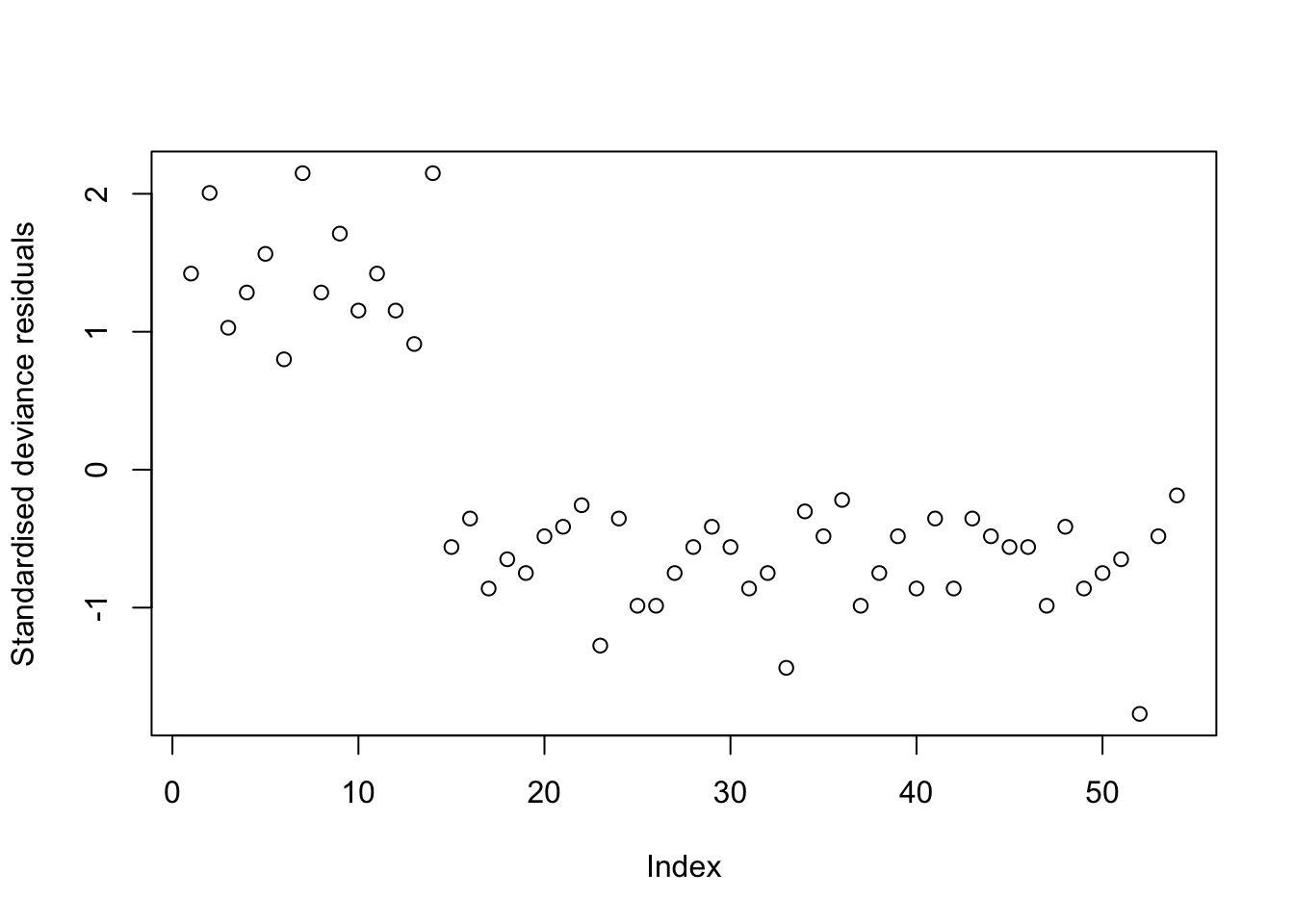
No standardised deviance residuals with values more extreme than –3 or 3, so it looks like we can be satisfied that the logistic regression model’s assumptions have been met.