sendata <- read_csv("https://uoepsy.github.io/data/SenilityWAIS.csv")
sen_mdl1 <- glm(senility ~ wais, family = "binomial", data = sendata)Diagnostics for influential observations
Just like in standard linear regression, we can check for influential observations using the measure of Cook’s Distance.
For logistic regression, the thresholds we typically use are the following:
- Cook’s Distance > 0.5 indicates moderately influential values.
- Cook’s Distance > 1 indicates highly influential values.
Let’s check for influential observations in our senility symptoms example:
To get the Cook’s Distance of each observation, we can use cooks.distance():
cooks.distance(sen_mdl1) 1 2 3 4 5 6 7 8
0.027667 0.092445 0.028824 0.028025 0.030689 0.022814 0.139247 0.028025
9 10 11 12 13 14 15 16
0.040386 0.029020 0.027667 0.029020 0.026683 0.139247 0.002517 0.001085
17 18 19 20 21 22 23 24
0.005820 0.003123 0.004010 0.001985 0.001501 0.000507 0.038345 0.001085
25 26 27 28 29 30 31 32
0.010022 0.010022 0.004010 0.002517 0.001501 0.002517 0.005820 0.004010
33 34 35 36 37 38 39 40
0.072744 0.000754 0.001985 0.000331 0.010022 0.004010 0.001985 0.005820
41 42 43 44 45 46 47 48
0.001085 0.005820 0.001085 0.001985 0.002517 0.002517 0.010022 0.001501
49 50 51 52 53 54
0.005820 0.004010 0.003123 0.210025 0.001985 0.000211 We can visually assess these values by specifying which = 4 when plotting your fitted model (i.e., plot(model, which = 4).
plot(sen_mdl1, which = 4)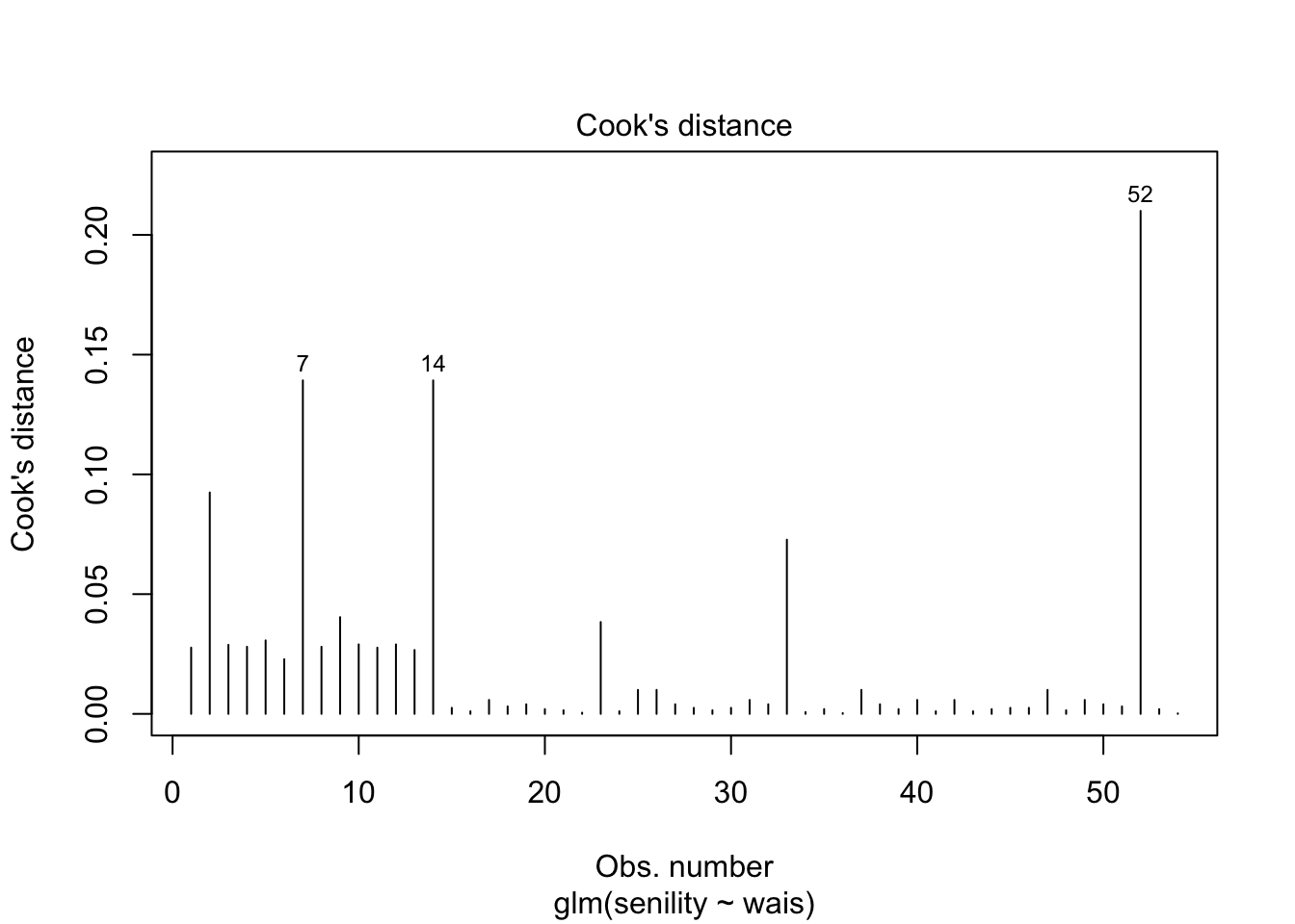
All observations have Cook’s Distance values below 0.5, so we have no unduly influential observations in this analysis.