By default, the contrast coding scheme that R uses is treatment coding.
It’s easiest to see how it works using examples.
Research Question
Does sepal length differ significantly between iris species?
Example: Binary predictor
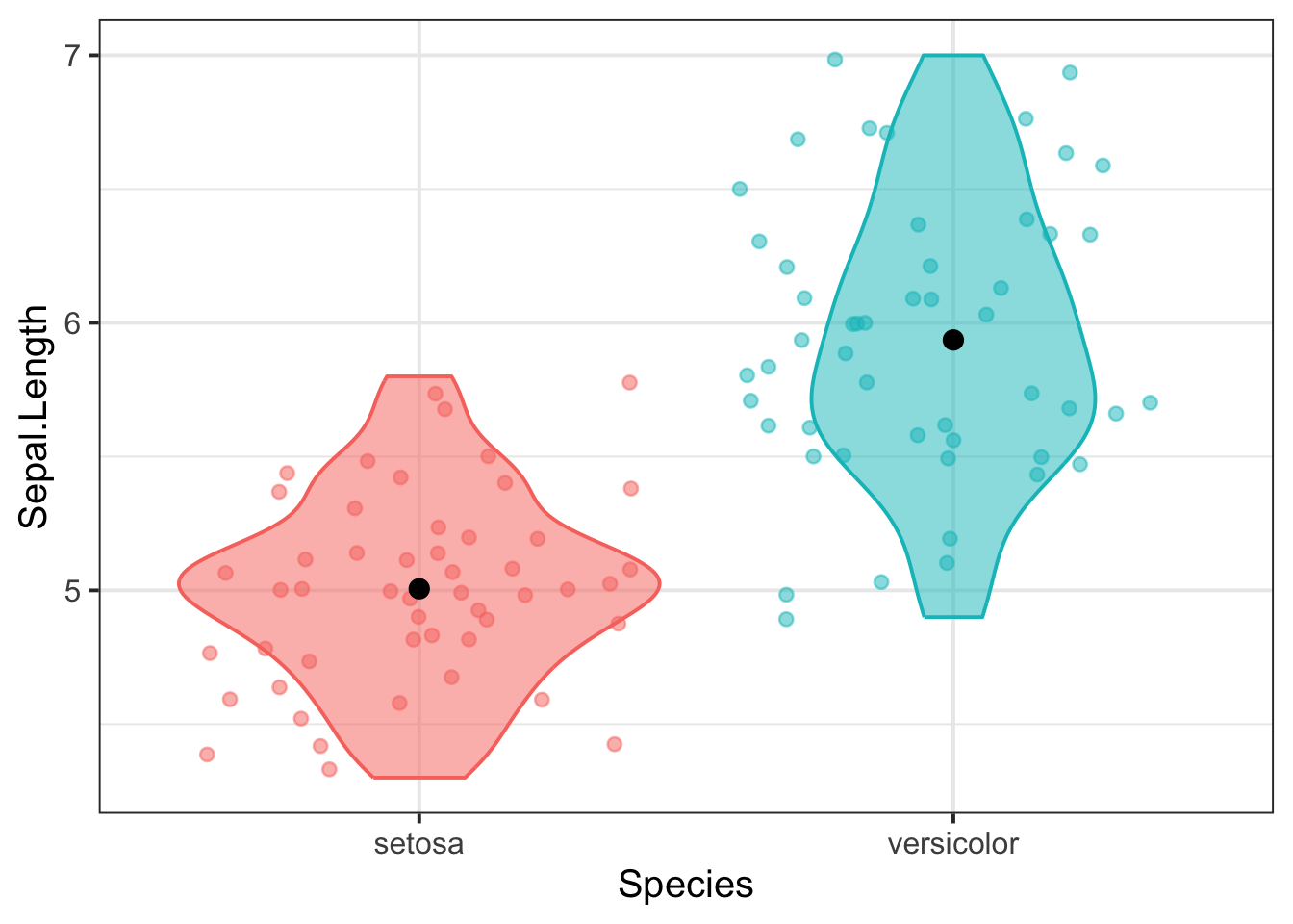
You have been provided with the in-built dataset, iris, which contains information concerning the sepal length (in cm), sepal width (in cm), petal length (in cm), and petal width (in cm) from three different species of iris (setosa, versicolor, and virginica). There are measurements for 50 flowers from each of the iris species (i.e., total \(n\) = 150). For this example, we’ll just look at two species, setosa and versicolor.
iris_binary <- iris |># filter out virginicafilter(Species !='virginica') |># the only factor levels we want are the two species we're keepingmutate(Species =factor(Species, levels =c('setosa', 'versicolor')))head(iris_binary)
We can see how R uses treatment coding to represent this variable using contrasts():
contrasts(iris_binary$Species)
           versicolor
setosa              0
versicolor          1
(If this code doesn’t run for your variable, then you’ll probably need to convert your variable to a factor using factor()).
This contrast matrix shows us that setosa is represented as 0, and versicolor is represented as 1. This means that setosa is the reference level, and versicolor is the non-reference level.
When we fit a linear model to this data, the model’s intercept will represent the estimated mean sepal length for the reference level setosa. And the model’s slope over Species will represented the estimated difference between the mean sepal length for versicolor and the mean sepal length for setosa. Or, in other words, how sepal length changes when we move from setosa (reference level) to versicolor (non-reference level).
Model fit and interpretation
m1 <-lm(Sepal.Length ~ Species, data = iris_binary)summary(m1)
Call:
lm(formula = Sepal.Length ~ Species, data = iris_binary)

Residuals:
   Min     1Q Median     3Q    Max
-1.036 -0.314 -0.006  0.272  1.064

Coefficients:
                  Estimate Std. Error t value Pr(>|t|)
(Intercept)         5.0060     0.0625    80.1   <2e-16 ***
Speciesversicolor   0.9300     0.0884    10.5   <2e-16 ***
---
Signif. codes:  0 '***' 0.001 '**' 0.01 '*' 0.05 '.' 0.1 ' ' 1

Residual standard error: 0.442 on 98 degrees of freedom
Multiple R-squared:  0.53,  Adjusted R-squared:  0.526
F-statistic:  111 on 1 and 98 DF,  p-value: <2e-16
The intercept is 5.01 cm, which corresponds to the mean sepal length of setosa:
Read this contrast matrix as a table with three rows and two columns.
The reference level is setosa. We can tell because its row contains only 0s.
There are two columns, which represent two “dummy variables”. Each dummy variable will estimate the difference between the reference level and the level that’s named in the column header and represented in that column as 1.
So the column versicolor contains a dummy variable that will compare versicolor to setosa, and the column virginica contains another dummy variable that will copmare virginica to setosa.
When we use Species as a predictor in a model, each dummy variable will receive its own coefficient in the model summary. That coefficient represents the comparisons described for each dummy variable.
Model fit and interpretation
m2 <-lm(Sepal.Length ~ Species, data = iris)summary(m2)
Call:
lm(formula = Sepal.Length ~ Species, data = iris)

Residuals:
   Min     1Q Median     3Q    Max
-1.688 -0.329 -0.006  0.312  1.312

Coefficients:
                  Estimate Std. Error t value Pr(>|t|)
(Intercept)         5.0060     0.0728   68.76  < 2e-16 ***
Speciesversicolor   0.9300     0.1030    9.03  8.8e-16 ***
Speciesvirginica    1.5820     0.1030   15.37  < 2e-16 ***
---
Signif. codes:  0 '***' 0.001 '**' 0.01 '*' 0.05 '.' 0.1 ' ' 1

Residual standard error: 0.515 on 147 degrees of freedom
Multiple R-squared:  0.619, Adjusted R-squared:  0.614
F-statistic:  119 on 2 and 147 DF,  p-value: <2e-16
The intercept is the mean estimated sepal length for the reference level setosa.
# A tibble: 3 x 2
  Species        m
  <fct>      <dbl>
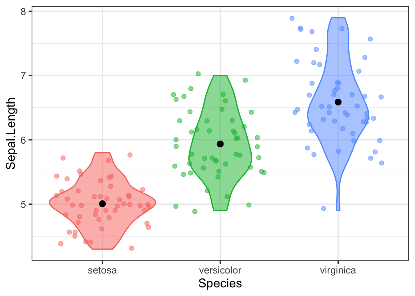
1 setosa      5.01
2 versicolor  5.94
3 virginica   6.59
The slope coefficient Speciesversicolor is 0.93, which is the difference between the mean estimated sepal length for versicolor (the non-reference level for this dummy variable) and that of setosa (the reference level).
5.94-5.01
[1] 0.93
And the slope coefficient Speciesvirginica is 1.58, which is the difference between the mean estimated sepal length for virginica (the non-reference level for this dummy variable) and that of setosa (the reference level).
6.59-5.01
[1] 1.58
Plotting model-fitted values
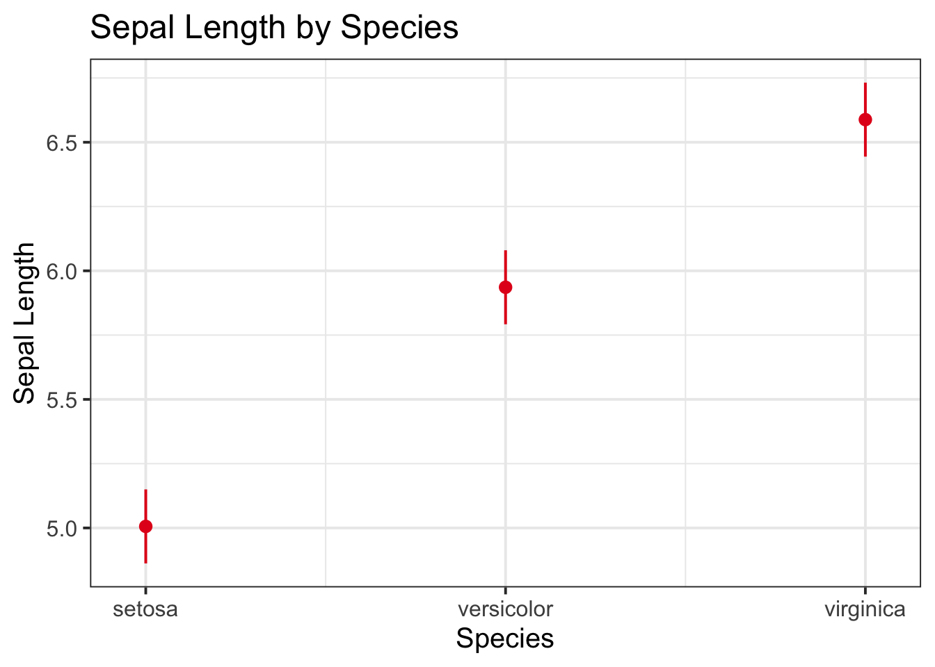
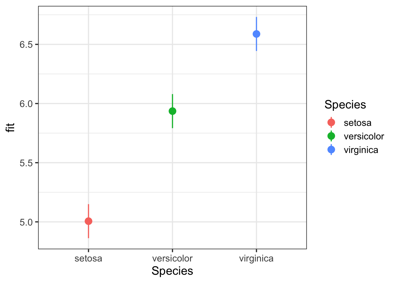
There are a couple of ways that we can visualise a model of categorical predictors, either using the sjPlot or effects packages:
library(sjPlot)plot_model(m2,type ="eff",terms ="Species") +labs(title ="Sepal Length by Species",x ="Species", y ="Sepal Length")
library(effects)effect(term =c("Species"), mod = m2) |>as.data.frame() |>ggplot(aes(x = Species, y = fit, col = Species)) +geom_pointrange(aes(ymin = lower, ymax = upper))
Reporting treatment coding (three-level example)
Dummy variables
$$
\text{Species}_\text{Versicolor} = \begin{cases}
1 & \text{if Species is Versicolor} \\
0 & \text{otherwise}
\end{cases}
$$
\[
\text{Species}_\text{Versicolor} = \begin{cases}
1 & \text{if Species is Versicolor} \\
0 & \text{otherwise}
\end{cases}
\]
$$
\text{Species}_\text{Virginica} = \begin{cases}
1 & \text{if Species is Virginica} \\
0 & \text{otherwise}
\\
\end{cases}
$$
\[
\text{Species}_\text{Virginica} = \begin{cases}
1 & \text{if Species is Virginica} \\
0 & \text{otherwise}
\\
\end{cases}
\]
$$
(\text{Species}_\text{Setosa } \text{ is the reference level})
$$
\[
(\text{Species}_\text{Setosa } \text{ is the reference level})
\]
For all coefficients, linear models always test the null hypothesis that the coefficient is equal to zero.
More specifically, for the mathematical model specified above:
For the intercept: the null hypothesis H0 is that the estimated mean outcome value for the reference level is equal to zero. The alternative hypothesis H1 is that the estimated mean outcome is different from zero. (This isn’t usually interesting to test, because the intercept will nearly always be different from zero.)
For a single slope coefficient (let’s say \(\beta_1\)): the null hypothesis is that the difference between the \(\beta_1\)’s non-reference level and the reference level is equal to zero. And the alternative hypothesis is that the difference between \(\beta_1\)’s non-reference level and the reference level is different from zero.
For all slope coefficients: the null hypothesis is that the differences between all non-reference levels and the reference level are equal to zero. And the alternative hypothesis is that any difference between any non-reference level and the reference level is different from zero.
Choose your contrast coding scheme based on the hypotheses you want to test.
For example: If your RQ asks whether two groups are significantly different, this question can be tested by looking at a slope coefficient of a treatment-coded categorical predictor.
Changing reference level
By default, R will always use the alphabetically first level as the reference level.
Imagine we wanted our reference level to be versicolor instead of setosa. R has a few equivalent options, so you can choose your favourite.
factor() (put the desired reference level first within c(), and the order of the others doesn’t matter; this is Elizabeth’s go-to because it’s the clearest and most generalisable):
Imagine you’d changed the contrast coding scheme of a predictor to something else, but you want to revert it back to treatment coding. Use the function contr.treatment() and specify the number of levels that the categorical variable has.