Mean-centering predictors

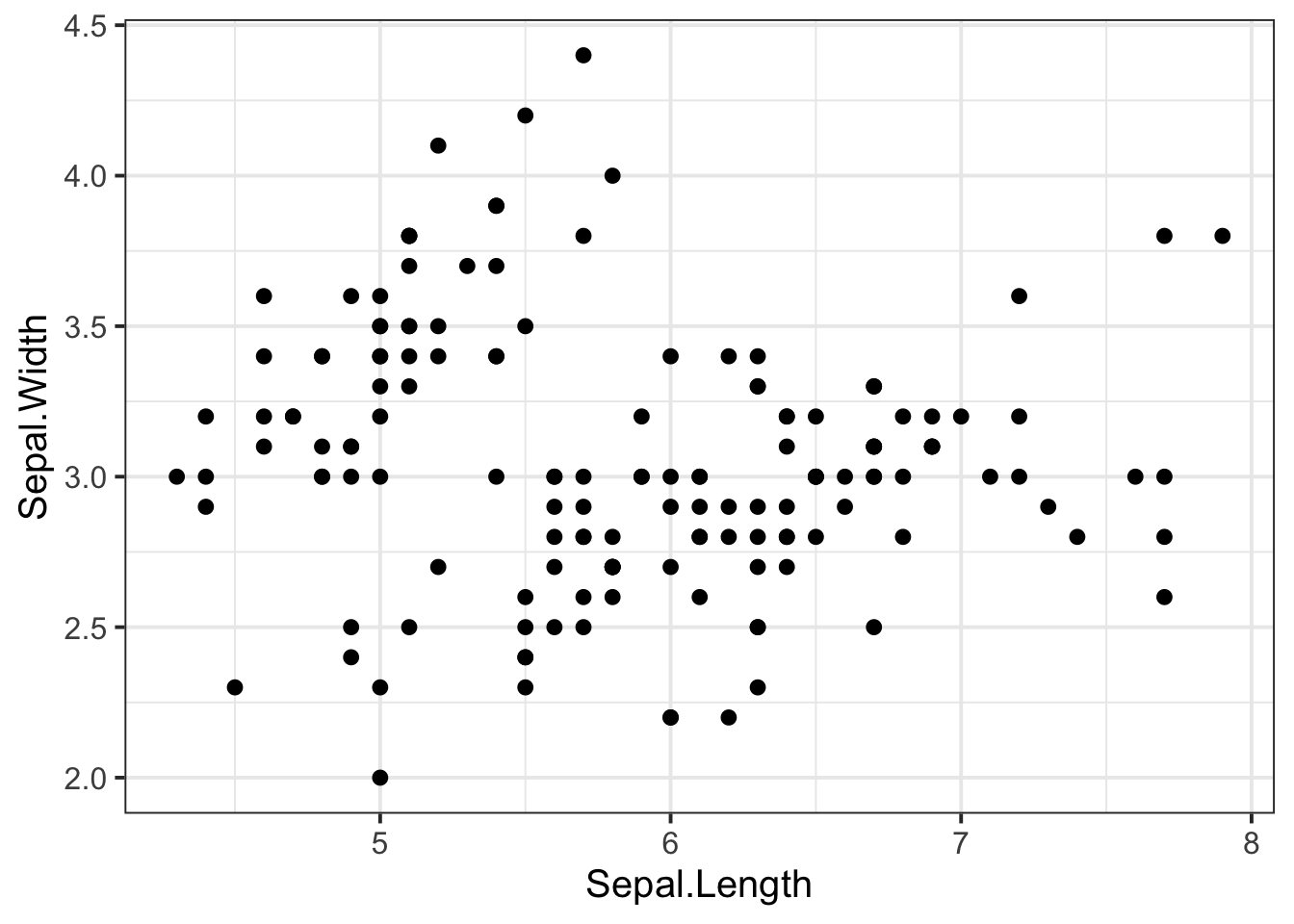
Mean-centering a variable is a transformation that shifts the variable so that whatever its mean used to be is now equal to zero. In other words, the variable is now centered on its mean.

How to mean-centre

To illustrate, here’s some data from the built-in iris dataset, comparing flowers’ sepal length to their sepal width:

iris |>
  ggplot(aes(x = Sepal.Length, y = Sepal.Width)) +
  geom_point()

Let’s imagine we want to mean-centre Sepal.Length.

To do so, we subtract the mean sepal length from every observation.

iris <- iris |>
  mutate(
    Sepal.Length_c = Sepal.Length - mean(Sepal.Length)
  )

Sense check that the mean of the new variable is indeed equal to zero:

mean(iris$Sepal.Length_c)

[1] -4.32e-16

For computational reasons, this check often produces a really really small decimal number. So it’s more useful to round it to the nearest integer and make sure that that value is zero.

mean(iris$Sepal.Length_c) |> round()

[1] 0

To illustrate, here’s a plot of the two versions of this variable side by side. In this plot, you can see the zero point of each version of the variable (the vertical red line).

Mean-centering causes the data to be shifted to the left, to become centered on the mean of zero. Below-average values are now negative, and above-average values are now positive.

Code

p_asis <- iris |>
  ggplot(aes(x = Sepal.Length, y = Sepal.Width)) +
  geom_point() +
  xlim(-2, 8) +
  geom_vline(xintercept = 0, colour = 'red') +
  ggtitle('Not mean-centred')

p_mc <- iris |>
  ggplot(aes(x = Sepal.Length_c, y = Sepal.Width)) +
  geom_point() +
  xlim(-2, 8) +
  geom_vline(xintercept = 0, colour = 'red') +
  ggtitle('Mean-centered')

p_asis + p_mc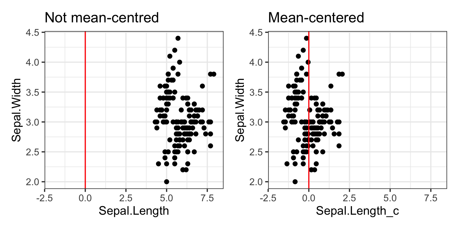

Why mean-centre a predictor?

When the zero point of a variable is nonsensical and/or impossible.
- Examples: height, shoe size
When zero is a possible value for the variable, but the data contain no observations where the value of the predictor equals zero (because then all the interpretations of the other coefficients that set the given predictor to zero are more unintuitive)
- Examples: Sepal.Length above, or (in many studies) age