library(palmerpenguins)Categorical/categorical example
RQ: Do differences in body mass between species differ by sex?
Here we are using the palmer penguins dataset1. The dataset contains a variety of information for a total of 344 adult penguins, including body measurements (bill length (bill_length_mm; measured in mm)/depth (bill_length_mm; measured in mm), flipper length (flipper_length_mm; measured in mm), body mass (body_mass_g; measured in grams)) for male and female (sex) penguins from three species (species; categorised as Adelie, Chinstrap, or Gentoo) across three Antarctic islands (island; categorised as Biscoe, Dream, or Torgersen) from 2007-2009 (year).
The variables we’ll use to address the RQ are body_mass_g, species, and sex.
Summarise/describe data
We can summarise the continuous outcome variables, grouped by the two categorical predictor variables, as follows.
penguins |>
  group_by(species, sex) |>
  summarise(
    BodyMass_M  = mean(body_mass_g),
    BodyMass_SD = sd(body_mass_g),
  ) |>
  drop_na() |> # some rows have missing values – comment out this line and see what changes!
  kableExtra::kable(
    caption = "Descriptive statistics for body mass (in g) for different penguin species and different sexes",
    digits = 2
  ) |>
kableExtra::kable_styling(full_width = FALSE)| species | sex | BodyMass_M | BodyMass_SD |
|---|---|---|---|
| Adelie | female | 3369 | 269 |
| Adelie | male | 4043 | 347 |
| Chinstrap | female | 3527 | 285 |
| Chinstrap | male | 3939 | 362 |
| Gentoo | female | 4680 | 282 |
| Gentoo | male | 5485 | 313 |
Visualise data
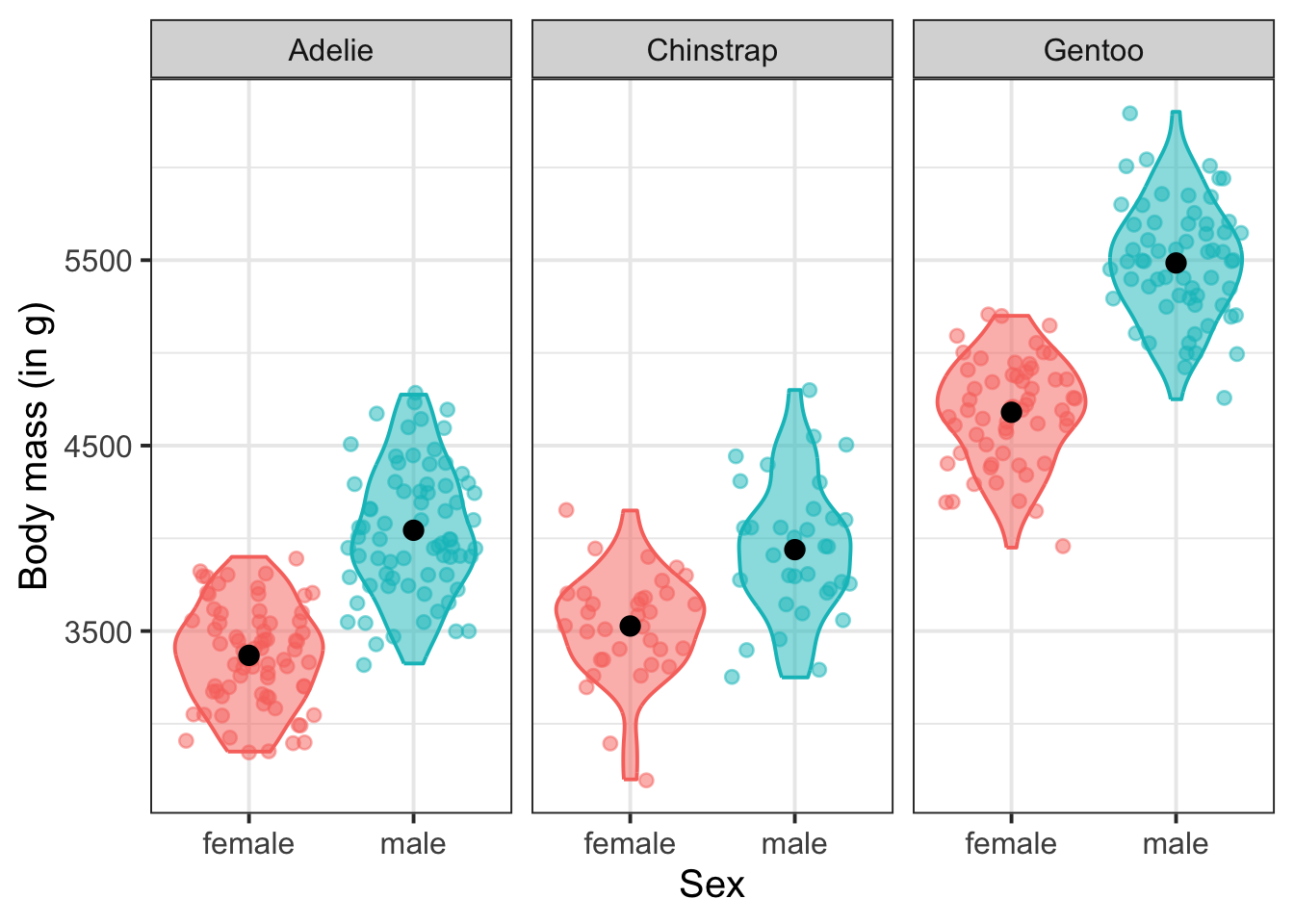
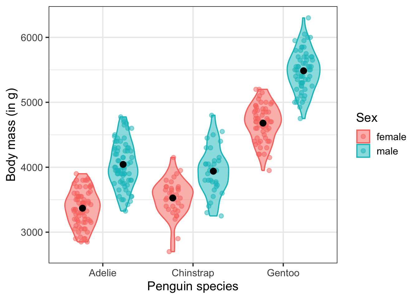
To plot a continuous outcome based on two categorical predictors, we can use violin plots again to plot the first predictor against the outcome, and distinguish levels of the second predictor using either facets or colour.
Facetting by species, colouring by sex (try it yourself facetting by sex and colouring by species instead):
penguins |>
  drop_na() |>  # drop any rows containing NAs
  ggplot(aes(x = sex, y = body_mass_g, fill = sex, colour = sex)) +
  geom_violin(alpha = 0.5) +
  geom_jitter(alpha = 0.5) +
  stat_summary(fun = mean, geom = 'point', colour = 'black', size = 3) +
  theme(legend.position = 'none') +
  facet_wrap(~ species) +
  labs(
    y = 'Body mass (in g)',
    x = 'Sex',
  )
Only colouring by sex (try it yourself colouring by species instead):
penguins |>
  drop_na() |>  # drop any rows containing NAs
  ggplot(aes(x = species, y = body_mass_g, fill = sex, colour = sex)) +
  geom_violin(alpha = 0.5) +
  geom_point(
      alpha = 0.5,
      position = position_jitterdodge(dodge.width = 0.9)  # align points + violins
  ) +
  stat_summary(
      fun = mean,
      geom = 'point',
      colour = 'black',
      show.legend = F,  # drop from legend
      size = 3,
      position = position_dodge(width = 0.9)  # align means + violins
  ) +
  labs(
    y = 'Body mass (in g)',
    x = 'Penguin species',
    fill = 'Sex',
    colour = 'Sex'
  )
Set up predictors
Before we specify our model, we must select (and provide justification for this choice) the reference group(s) for our categorical variable(s).
In this specific example, there is no natural reference category, nor one that maps to our RQ, so we will go with R’s default coding and have Adelie as our reference group for species, and female for sex.
contrasts(penguins$species) Chinstrap Gentoo
Adelie 0 0
Chinstrap 1 0
Gentoo 0 1contrasts(penguins$sex) male
female 0
male 1How many interaction terms will the model contain?
The number of interaction terms is given by
\[ (r - 1) \times (c - 1) \]
- \(r\) (which stands for “rows”) is the number of levels in the first interacting predictor;
- \(c\) (which stands for “columns”) is the number of levels in the second interacting predictor.
To see why we are talking about “rows” and “columns”, imagine the variables arranged in a table like this:
| female | male | |
|---|---|---|
| Adelie | … | … |
| Chinstrap | … | … |
| Gentoo | … | … |
So in our 3x2 data, where \(r=3\) and \(c=2\), we have
\[ \begin{align} & (r - 1) \times (c - 1)\\ =~& (3 - 1) \times (2 - 1) \\ =~& 2 \times 1 \\ =~& 2 \end{align} \]
interaction terms.
Mathematical model specification
\[ \begin{align} \text{body\_mass\_g} ~=~ & \beta_0 + (\beta_1 \cdot \text{species}_\text{Chinstrap}) + (\beta_2 \cdot \text{species}_\text{Gentoo}) + (\beta_3 \cdot \text{sex}_\text{male}) ~+ \\ & (\beta_4 \cdot \text{species}_\text{Chinstrap} \cdot \text{sex}_\text{male}) + (\beta_5 \cdot \text{species}_\text{Gentoo} \cdot \text{sex}_\text{male}) + \epsilon \end{align} \]
Write:
$$
\begin{align}
\text{body\_mass\_g} ~=~ & \beta_0 +
(\beta_1 \cdot \text{species}_\text{Chinstrap}) +
(\beta_2 \cdot \text{species}_\text{Gentoo}) +
(\beta_3 \cdot \text{sex}_\text{male}) ~+  \\
& (\beta_4 \cdot \text{species}_\text{Chinstrap} \cdot \text{sex}_\text{male}) +
(\beta_5 \cdot \text{species}_\text{Gentoo} \cdot \text{sex}_\text{male}) +
\epsilon
\end{align}
$$
H0 and H1
For most RQs that require interaction models, we’re interested in testing the hypothesis that there’s no difference in how some predictor x is associated with the outcome y for different values of z. In other words, we are interested in testing the null hypothesis that the interaction term is zero.
For the model above:
\[ \begin{align} H_0 &: \text{All } \beta_j = 0 \text{ for } j = 4, 5\\ H_1 &: \text{Any } \beta_j \neq 0\\ \end{align} \]
Write:
$$
\begin{align}
H_0 &: \text{All } \beta_j = 0 \text{ for } j = 4, 5\\
H_1 &: \text{Any } \beta_j \neq 0\\
\end{align}
$$
Fit the model
mdl_cc <- lm(body_mass_g ~ species * sex, data = penguins)Each row in the summary() output of the model will correspond to one of the estimated \(\beta\)’s in the equation above.
summary(mdl_cc)
Call:
lm(formula = body_mass_g ~ species * sex, data = penguins)

Residuals:
   Min     1Q Median     3Q    Max
  -827   -214     11    206    861

Coefficients:
                         Estimate Std. Error t value Pr(>|t|)
(Intercept)                3368.8       36.2   93.03   <2e-16 ***
speciesChinstrap            158.4       64.2    2.47   0.0142 *
speciesGentoo              1310.9       54.4   24.09   <2e-16 ***
sexmale                     674.7       51.2   13.17   <2e-16 ***
speciesChinstrap:sexmale   -262.9       90.8   -2.89   0.0041 **
speciesGentoo:sexmale       130.4       76.4    1.71   0.0889 .
---
Signif. codes:  0 '***' 0.001 '**' 0.01 '*' 0.05 '.' 0.1 ' ' 1

Residual standard error: 309 on 327 degrees of freedom
  (11 observations deleted due to missingness)
Multiple R-squared:  0.855, Adjusted R-squared:  0.852
F-statistic:  384 on 5 and 327 DF,  p-value: <2e-16
Interpret results
\(\beta_0\) = (Intercept) = 3368.84
- A female Adelie penguin is expected to have a body mass of 3368.84 g.
\(\beta_1\) = speciesChinstrap = 158.37
- A female Chinstrap penguin is estimated to have a body mass 158.37 g greater than a female Adelie penguin.
- This estimate is significantly different from zero \((p = .014)\).
\(\beta_2\) = speciesGentoo = 1310.91
- A female Gentoo penguin is estimated to have a body mass 1310.91 g greater than a female Adelie penguin.
- This estimate is significantly different from zero \((p < .001)\).
\(\beta_3\) = sexmale = 674.66
- A male Adelie penguin is estimated to have a body mass 674.66 g greater than a female Adelie penguin.
- This estimate is significantly different from zero \((p < .001)\).
\(\beta_4\) = speciesChinstrap:sexmale = -262.89
- For Chinstrap penguins, the difference between male and female penguins is estimated to decrease by 262.9 g compared to the male/female difference for Adelie penguins.
- This estimate is significantly different from zero \((p = .004)\).
\(\beta_5\) = speciesGentoo:sexmale = 130.44
- For Gentoo penguins, the difference between male and female penguins is estimated to increase by 130.44 g compared to the male/female difference for Adelie penguins.
Visualise the model
We can do this using the cat_plot() function from the interactions package.
In terms of of specification, it might be useful to look up the helper function (i.e., ?cat_plot). As a quick guide:
model =: The name model to be used
pred =: The categorical predictor variable that will appear on the x-axis
modx =: The categorical moderator variable
Remember to give your plot informative titles/labels. You, for example, likely want to give your plot:
- a clear and concise title (specify
main.title =)
- axis labels with units or scale included (specify
x.label =andy.label =)
- a legend title (specify
legend.main =)
library(interactions)

plt_mdl_cc <- cat_plot(
  model = mdl_cc,
  pred = species,
  modx = sex,
  main.title = "Body mass across species and sex",
  x.label = "Species",
  y.label = "Body mass (in g)",
  legend.main = "Sex"
)
plt_mdl_cc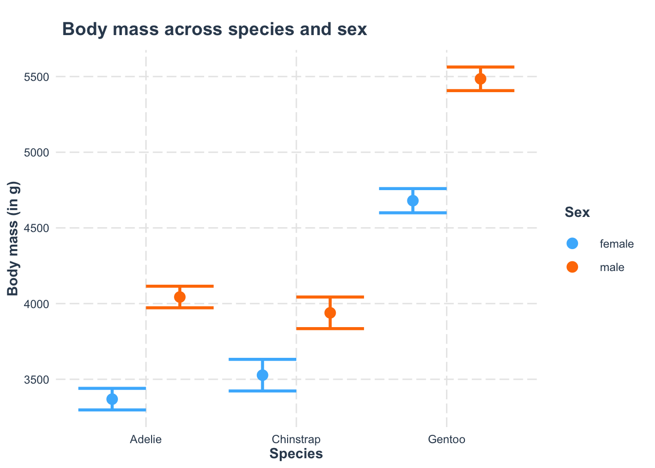
Testing simple effects
probe_interactions() would test simple slopes for continuous predictors, but it doesn’t work quite the same way for categorical predictors, so we need some new machinery. Specifically, we’ll use the emmeans package and its function emmeans().
library(emmeans)Imagine we want to find the simple effects of sex for each species of penguin: that is, how much do males and females differ for Adelie penguins, and for Chinstrap penguins, and for Gentoo penguins, and are each of those differences significantly different from zero?
You can run this analysis step by step:
# Use `emmeans()` to get estimated body mass
# for all combinations of species and sex
mdl_cc_emm <- emmeans(mdl_cc, ~ species * sex)

## Use `pairs()` to find the simple effects of sex for each species
pairs(mdl_cc_emm, simple = "sex")
species = Adelie:
contrast estimate SE df t.ratio p.value
female - male -675 51.2 327 -13.170 <0.0001
species = Chinstrap:
contrast estimate SE df t.ratio p.value
female - male -412 75.0 327 -5.490 <0.0001
species = Gentoo:
contrast estimate SE df t.ratio p.value
female - male -805 56.7 327 -14.190 <0.0001Or you can do the same analysis all in one command:
pairs(
  emmeans(mdl_cc, ~ species * sex),
  simple = "sex"
)
species = Adelie:
contrast estimate SE df t.ratio p.value
female - male -675 51.2 327 -13.170 <0.0001
species = Chinstrap:
contrast estimate SE df t.ratio p.value
female - male -412 75.0 327 -5.490 <0.0001
species = Gentoo:
contrast estimate SE df t.ratio p.value
female - male -805 56.7 327 -14.190 <0.0001In this case, the differences between males and females for all penguin species are significantly different from zero.
Footnotes
Horst, A. M., Hill, A. P., & Gorman, K. B. (2020). palmerpenguins: Palmer Archipelago (Antarctica) penguin data. R package version 0.1.0. https://allisonhorst.github.io/palmerpenguins/ doi: 10.5281/zenodo.3960218↩︎